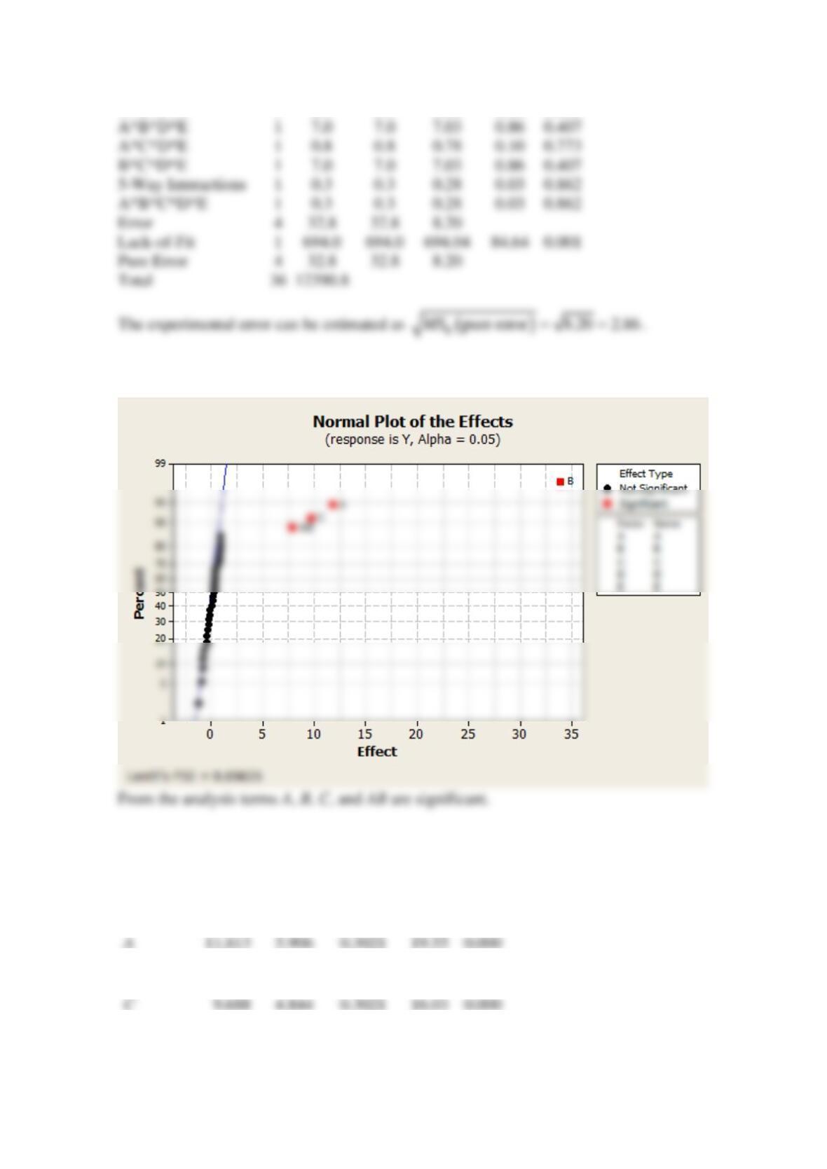
A*B*C*D
1
0.0
0.0
0.03
0.00
0.954
A*B*C*E
1
0.3
0.3
0.28
0.03
0.862
Pooling out nonsignificant effects:
Factorial Fit: y versus A, B, C, and AB.
Estimated Effects and Coefficients for y (coded units)
Term
Effect
Coef
SE Coef
T
P
Constant
30.531
0.3021
101.70
0.000
A
11.813
5.906
0.3021
19.55
0.000
B
33.937
16.969
0.3021
56.17
0.000
C
9.688
4.844
0.3021
16.03
0.000
AB
7.938
3.969
0.3021
13.14
0.000
A*B*D*E
1
7.0
7.0
7.03
0.86
0.407
A*C*D*E
1
0.8
0.8
0.78
0.10
0.773
B*C*D*E
1
7.0
7.0
7.03
0.86
0.407
5-Way Interactions
1
0.3
0.3
0.28
0.03
0.862
A*B*C*D*E
1
0.3
0.3
0.28
0.03
0.862
Error
4
32.8
32.8
8.20
Lack-of-Fit
1
694.04
0.001
Pure Error
4
32.8
32.8
8.20
Total
Analysis of Variance for y (coded units)
Source
DF
Seq SS
Adj SS
Adj MS
F
P
Main Effects
3
11081.1
11081.1
3693.70
1264.90
0.000
2-Way Interactions
1
504.03
172.61
0.000
Residual Error
27
78.8
78.8
2.92
Lack of Fit
3
3.1
3.1
1.03
0.33
0.806
24
75.8
75.8
3.16
Total
31
11664.0
(b)
Reserve Problems Chapter 14 Section 7 Problem 3
An experiment to study the effect of machining factors on ceramic strength was described at
www.itl.nist.gov/div898/handbook/. Five factors were considered at two levels each: A denotes
Table Speed, B denotes Down Feed Rate, C denotes Wheel Grit, D denotes Direction, and E
denotes Batch. The response is the average of the ceramic strength over 15 repetitions. The
following data are from a single replicate of a
5
2
factorial design.
A
B
C
D
E
Strength
–1
–1
–1
–1
–1
680.45
1
–1
–1
–1
–1
722.48
–1
1
–1
–1
–1
702.14
1
1
–1
–1
–1
666.93
–1
–1
1
–1
–1
703.67
1
–1
1
–1
–1
642.14
–1
1
1
–1
–1
692.98
1
1
1
–1
–1
669.26
S = 1.70884 R-Sq = 99.32% R-Sq(adj) = 99.22%
–1
–1
–1
1
–1
491.58
1
–1
–1
1
–1
475.52
–1
1
–1
1
–1
478.76
1
1
–1
1
–1
568.23
–1
–1
1
1
–1
444.72
1
–1
1
1
–1
410.37
–1
1
1
1
–1
428.51
1
1
1
1
–1
491.47
–1
–1
–1
–1
1
607.34
1
–1
–1
–1
1
620.8
–1
1
–1
–1
1
610.55
1
1
–1
–1
1
638.04
–1
–1
1
–1
1
585.19
1
–1
1
–1
1
586.17
–1
1
1
–1
1
601.67
1
1
1
–1
1
608.31
–1
–1
–1
1
1
442.9
1
–1
–1
1
1
434.41
–1
1
–1
1
1
417.66
1
1
–1
1
1
510.84
–1
–1
1
1
1
392.11
1
–1
1
1
1
343.22
–1
1
1
1
1
385.52
1
1
1
1
1
446.73
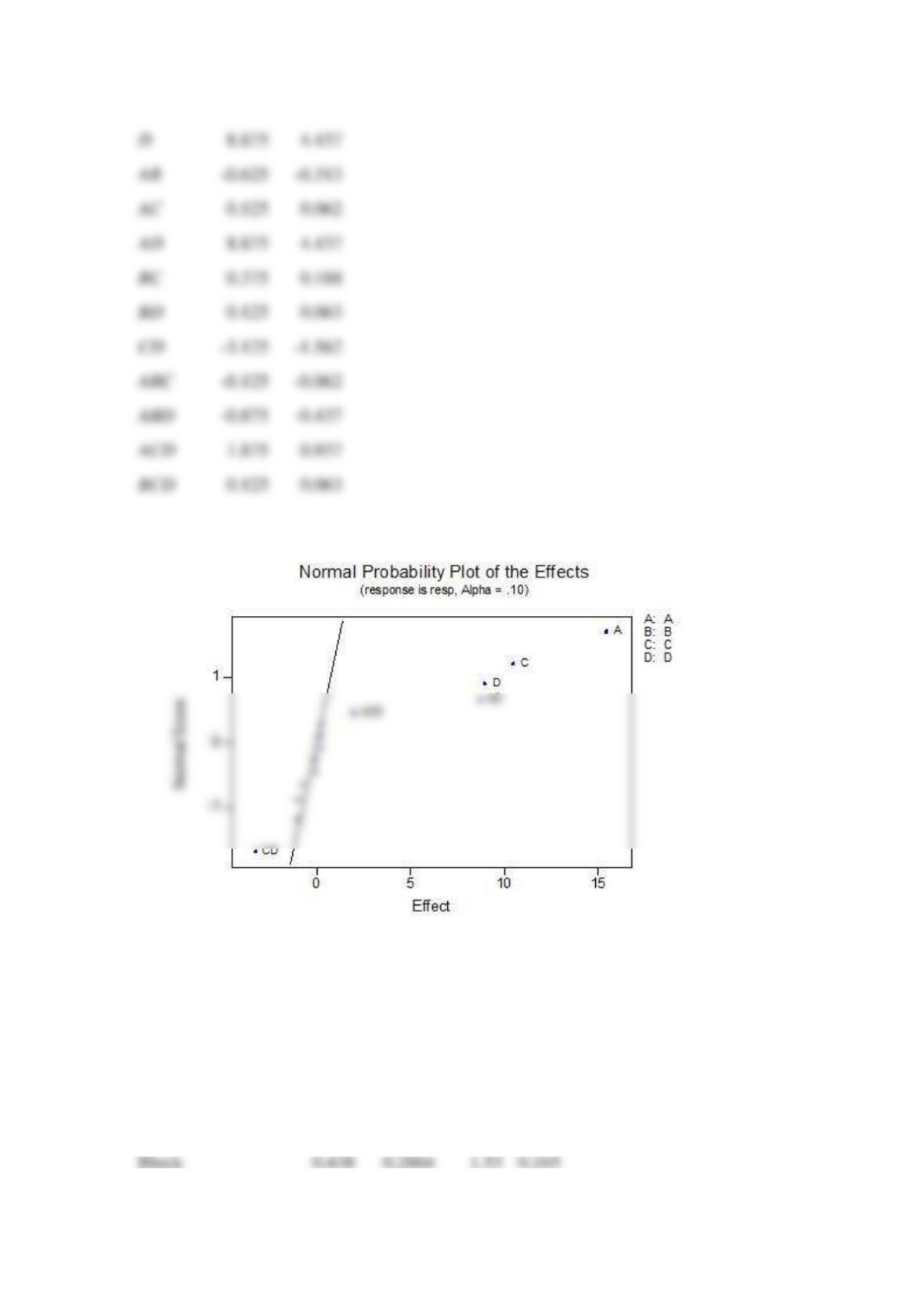
(a) Estimate the factor and use a normal probability plot of the effects. Identify which effects
appear to be large.
(b) Fit an appropriate model using the factors identified in part (a).
(c) Use residuals plots for strength. Is normality assumption reasonable?
(d) Identify the two largest interactions.
SOLUTION
(a)
Estimated Effects and Coefficients for Strength (coded units)
Term
Effect
Coef
Constant
546.90
A
10.57
5.29
B
20.91
10.45
C
-39.79
-19.89
D
-198.47
-99.24
E
-64.86
-32.43
AB
24.68
12.34
AC
-15.16
-7.58
AD
14.31
7.15
AE
7.62
3.81
BC
6.20
3.10
BD
15.70
7.85
BE
4.99
2.49
CD
-19.87
-9.93
CE
-1.92
-0.96
DE
12.89
6.44
ABC
6.68
3.34
ABD
27.15
13.57
ACD
0.51
0.26
ABE
4.25
2.13
ACE
1.95
0.97
ADE
-8.25
-4.13
BCD
-2.36
BCE
1.79
0.89
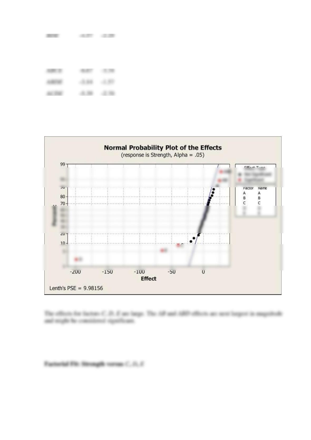
CDE
2.01
1.01
ABCD
-6.65
-3.33
ABDE
-3.14
-1.57
ACDE
-5.39
-2.70
BCDE
5.80
2.90
ABCDE
8.75
4.38
(b)
Estimated Effects and Coefficients for Strength (coded units)
Term
Effect
Coef
SE Coef
T
P
BDE
-4.57
-2.29
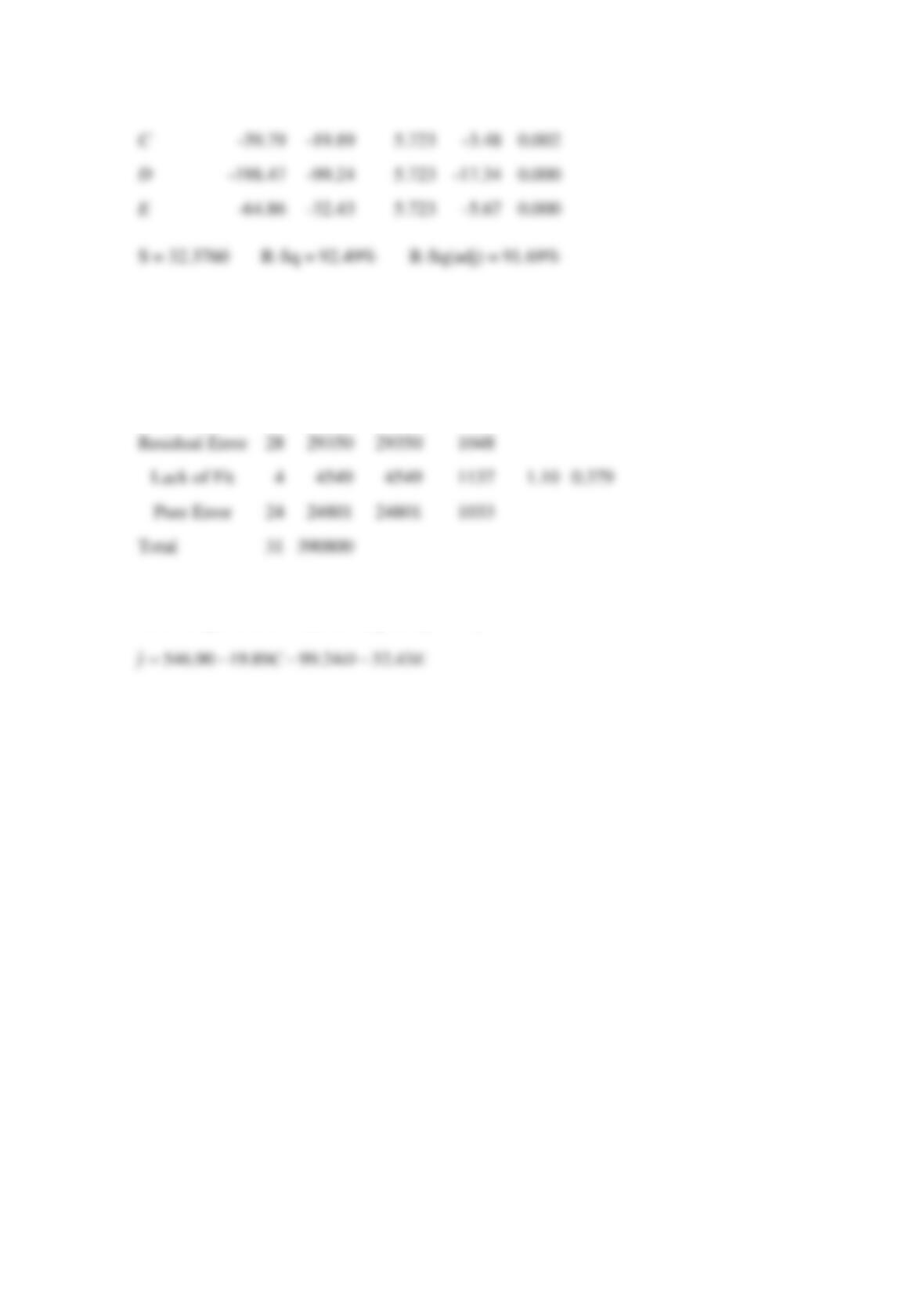
Constant
546.90
5.723
95.56
0.000
Analysis of Variance for y (coded units)
Source
DF
Seq SS
Adj SS
Adj MS
F
P
Main Effects
3
361451
361451
120484
114.94
0.000
Residual Error
28
4
0.379
24
Total
31
390800
The average of the ceramic strength is given by
(c)
-39.79
5.723
0.002
-198.47
5.723
-17.34
0.000
S = 32.3760 R-Sq = 92.49% R-Sq(adj) = 91.69%
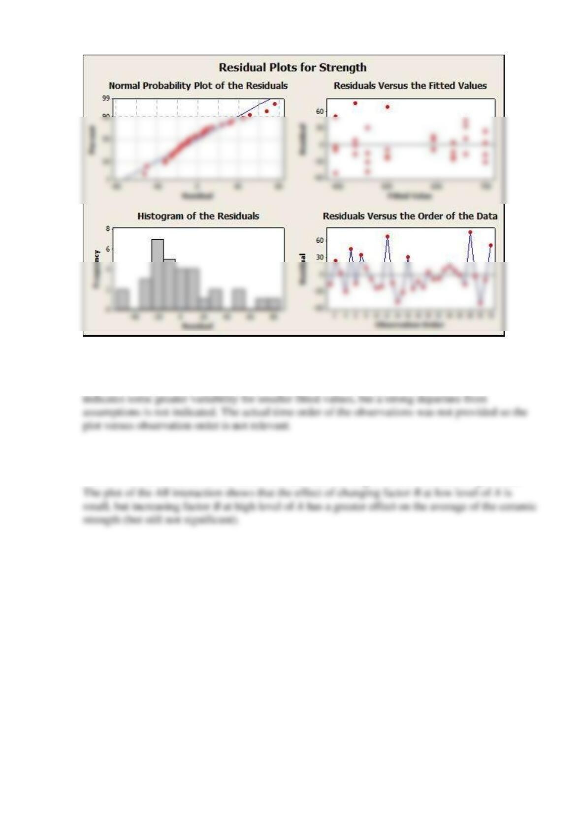
Is normality assumption reasonable?
The normality assumption is reasonable. The plot of residuals versus the predicted values
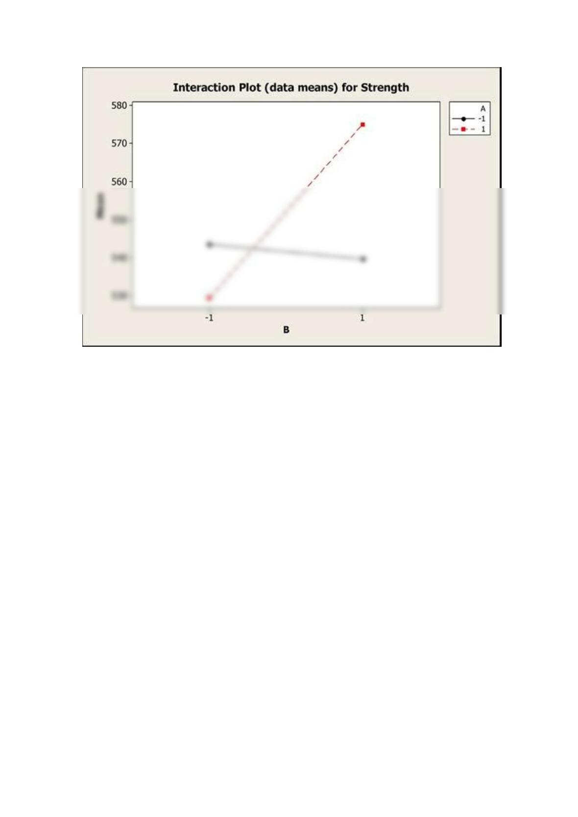
(d)
The two interaction terms in this model AB and ABD are large, but not considered significant.
Reserve Problems Chapter 14 Section 7 Problem 4
Consider the following computer output for a
3
2
factorial experiment.
Estimated Effects and Coefficients
Term
Effect
Coef
SE Coef
t
P
Constant
583.57
?
115.40
0.000
A
5.40
?
?
?
?
B
20.94
10.47
?
2.07
0.072
C
-41.73
-20.86
?
-4.13
0.003
A*B
26.93
13.46
?
2.66
0.029
A*C
-20.41
-10.20
?
-2.02
0.078
B*C
3.91
1.96
?
0.39
0.709
A*B*C
-12.07
-6.04
?
-1.19
0.267
S=20.2279
Analysis of Variance
Source
DF
SS
MS
F
P
A
?
?
?
?
?
B
?
1753.4
1753.40
4.29
0.072
C
?
6965.0
6964.95
17.02
0.003
A*B
?
2900.8
2900.76
7.09
0.029
A*C
?
1665.9
1665.93
4.07
0.078
B*C
?
61.3
61.25
0.15
0.709
A*B*C
?
583.1
583.06
1.42
0.267
Residual error
?
3273.4
409.17
Total
15
17319.5
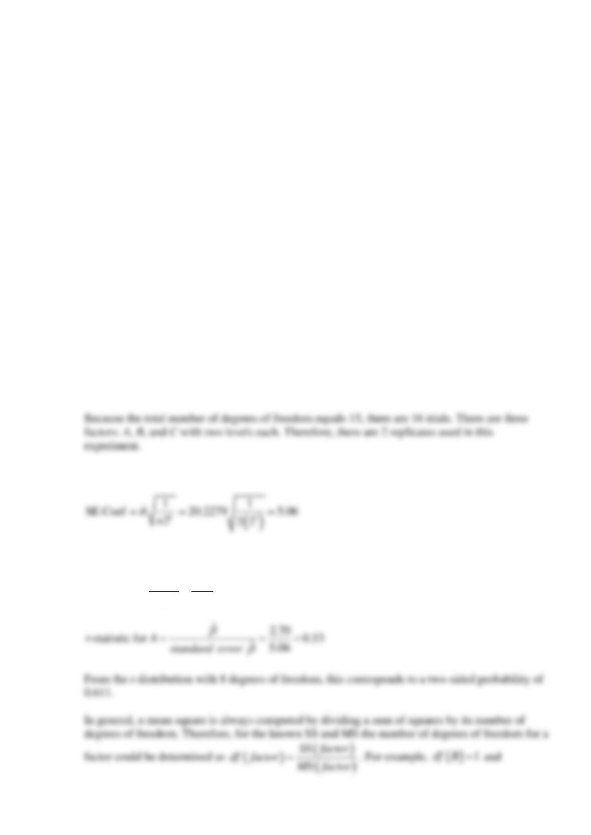
(a) How many replicates were used in the experiment?
(b) Use the appropriate equation to calculate the standard error of a coefficient.
(c) Calculate the entries marked with “?” in the output.
SOLUTION
(a)
(b)
(c)
5.40 2.70
22
Effect
Coef of A = = =
Reserve Problems Chapter 14 Section 7 Problem 5
The book Using Designed Experiments to Shrink Health Care Costs [1997, ASQ Quality Press]
presented a case study of an unreplicated
5
2
factorial design to investigate the effect of five
factors on the length of accounts receivable measured in days. A summary of the investigated
factors and the results of the study follows.
Row
Payer
Type
Number
of Visits
Disciplines
Length
of Stay
Case
Manager
Length of Account
Receivable (days)
1
−
−
−
−
−
17
2
+
−
−
−
−
28
3
−
+
−
−
−
40
4
+
+
−
−
−
31
5
−
−
+
−
−
5
6
+
−
+
−
−
28
7
−
+
+
−
−
43
8
+
+
+
−
−
47
9
−
−
−
+
−
26
10
+
−
−
+
−
29
11
−
+
−
+
−
60
12
+
+
−
+
−
47
13
−
−
+
+
−
18
14
+
−
+
+
−
32
15
−
+
+
+
−
64
16
+
+
+
+
−
49
17
−
−
−
−
+
33
18
+
−
−
−
+
31
19
−
+
−
−
+
67
20
+
+
−
−
+
79

21
−
−
+
−
+
32
22
+
−
+
−
+
46
23
−
+
+
−
+
86
24
+
+
+
−
+
55
25
−
−
−
+
+
41
26
+
−
−
+
+
63
27
−
+
−
+
+
77
28
+
+
−
+
+
197
29
−
−
+
+
+
62
30
+
−
+
+
+
52
31
−
+
+
+
+
143
32
+
+
+
+
+
68
Level
-1
1
Payer Type
Medicare
Risk Medicare
Number of visits
9
10
Disciplines
2
3c
Length of stay
30
31
Case manager
Registered Nurses
Physical Therapists
(a) Construct the normal probability plot of the effects to find significant main effects.
(b) Pool the negligible higher-order interactions to obtain an estimate of the error and construct
the ANOVA accordingly. Find the adjusted mean square of the error.
SOLUTION
(a)
(b)
Estimated Effects and Coefficients for length of account receivable (coded units)
Term
Effect
Coef
SE Coef
T
P
Constant
53.00
4.275
12.40
0.000
Number of visits
38.12
19.06
4.275
0.000
Length of stay
22.50
11.25
4.275
0.014
Case manager
35.50
17.75
4.275
0.000
S = 24.1823 PRESS = 21386.3
R-Sq = 61.14% R-Sq(pred) = 49.24% R-Sq(adj) = 56.97%
Analysis of Variance for length of account receivable (coded units)
Source
DF
Seq SS
Adj SS
Adj MS
F
P
Main Effects
8586.7
14.68
0.000
Length of stay
1
4050
4050
4050.0
6.93
0.014
Reserve Problems Chapter 14 Section 8 Problem 1
Four factors are thought to influence the taste of a soft-drink beverage: type of sweetener
( )
A
,
ratio of syrup to water
( )
B
, carbonation level
( )
C
, and temperature
( )
D
. Each factor can be run
at two levels, producing a
4
2
design. At each run in the design, samples of the beverage are
given to a test panel consisting of 20 people. Each tester assigns the beverage a point score from
1 to 10. Total score is the response variable, and the objective is to find a formulation that
maximizes total score. Two replicates of this design are run, and the results are shown in the
table.
Treatment
Combination
Replicate
I
II
( )
1
159
163
a
168
175
b
158
163
ab
166
168
c
175
178
ac
179
183
bc
173
168
abc
179
182
d
164
159
ad
187
189
bd
163
159
abd
185
191
cd
168
174
acd
197
199
bcd
170
174
1
10082.0
17.24
0.000
Residual Error
3530
3530
Pure Error
Total
abcd
194
198
Consider the data from the first replicate.
(a) Construct a design with two blocks of eight observations each with ABCD confounded.
(b) Analyze the data. Use
0.10
=
.
SOLUTION
(a)
Blocks
A
B
C
D
Rep I
1
-1
-1
-1
-1
159
1
-1
1
1
-1
173
1
1
-1
-1
1
187
1
-1
1
-1
1
163
1
-1
-1
1
1
168
1
1
1
1
1
194
2
1
-1
-1
-1
168
2
-1
1
-1
-1
158
2
-1
-1
1
-1
175
2
1
1
1
-1
179
2
-1
-1
-1
1
164
2
1
1
-1
1
185
2
1
-1
1
1
197
2
-1
1
1
1
170
(b)
Term
Effect
Coef
Block
A
15.625
7.813
B
1
1
1
-1
-1
166
1
1
-1
1
-1
179
C
10.625
5.312
Factors A, C, and D, and interactions AD, CD, and ACD appear to be significant.
Estimated Effects and Coefficients (coded units)
Term
Effect
Coef
SE Coef
T
P
Constant
174.063
0.2864
607.74
0.000
0.438
0.2864
1.53
0.165
A
15.625
7.812
0.2864
27.28
0.000
D
8.875
4.437
-0.625
8.875
4.437
0.375
0.188
0.125
0.063
-3.125
-0.125
-0.875
ACD
1.875
0.937
BCD
0.125
0.063
Reserve Problems Chapter 14 Section 8 Problem 2
Consider the following computer output from a single replicate of a
4
2
experiment in two blocks
with ABCD confounded.
Term
Effect
Coef
SE Coef
t
P
Constant
579.33
9.928
58.35
0
Block
105.68
9.928
10.64
0
A
-15.41
-7.7
9.928
-0.78
0.481
B
2.95
1.47
9.928
0.15
0.889
C
15.92
7.96
9.928
0.8
0.468
D
-37.87
-18.94
9.928
-1.91
0.129
A*B
-8.16
-4.08
9.928
-0.41
0.702
A*C
5.91
2.95
9.928
0.3
0.781
A*D
30.28
?
9.928
?
0.202
B*C
20.43
10.21
9.928
1.03
0.362
B*D
-17.11
-8.55
9.928
-0.86
0.437
C*D
4.41
2.21
9.928
0.22
0.835
S = 39.7131 R-Sq = 96.84% R-Sq (adj) = 88.16%
(a) What effects were used to generate the residual error in the ANOVA?
(b) Calculate the entries marked with “?” in the output.
SOLUTION
10.625
18.55
8.875
15.49
8.875
15.49
1.875
S = 1.14564 R-Sq = 99.51% R-Sq(adj) = 99.07%
(a)
The effects for all three-factor interaction terms (ABC, ABD, ACD, and BCD) are used to
(b)
Reserve Problems Chapter 14 Section 8 Problem 3
An article in Journal of Construction Engineering and Management (“Analysis of Earth-Moving
Systems Using Discrete—Event Simulation,” 1995, Vol. 121(4), pp. 388–396) considered a
replicated two-level factorial experiment to study the factors most important to output in an
earth-moving system. The experiment was handled as four replicates of a
4
2
factorial design
with response equal to production rate (m3/h). The data are shown in the following table.
Row
Number
of
Trucks
Passes
per Load
Load-
pass
Time
Travel
Time
Production (m3/h)
1
2
3
4
1
−
−
−
−
179.6
179.8
176.3
173.1
2
+
−
−
−
373.1
375.9
372.4
361.1
3
−
+
−
−
153.2
153.6
150.8
148.6
4
+
+
−
−
226.1
220
225.7
218.5
5
−
−
+
−
156.9
155.4
154.2
152.2
6
+
−
+
−
242
233.5
242.3
233.6
7
−
+
+
−
122.7
119.6
120.9
118.6
8
+
+
+
−
135.7
130.9
135.5
131.6
9
−
−
−
+
44.2
44
43.5
43.6
10
+
−
−
+
124.2
123.3
122.8
121.6
11
−
+
−
+
42
42.4
42.5
41
12
+
+
−
+
116.3
117.3
115.6
114.7
13
−
−
+
+
42.1
42.6
42.8
42.9
14
+
−
+
+
119.1
119.5
116.9
117.2
15
−
+
+
+
39.6
39.7
39.5
39.2
16
+
+
+
+
107
105.3
104.2
103
Level
-1
1
Number of trucks
2
6
Passes per load
4
7
Load-pass time
12 s
16 s
Travel time
100 s
800 s
The experiment actually used two different operators with the production in columns 1 and 3
from operator 1 and 2, respectively. Analyze the results from only columns 1 and 3 handled as
blocks.
(a) Assuming that the operator is a nuisance factor, estimate the factor effects.
(b) Based on a normal probability plot of the effect estimates, identify a model for the data from
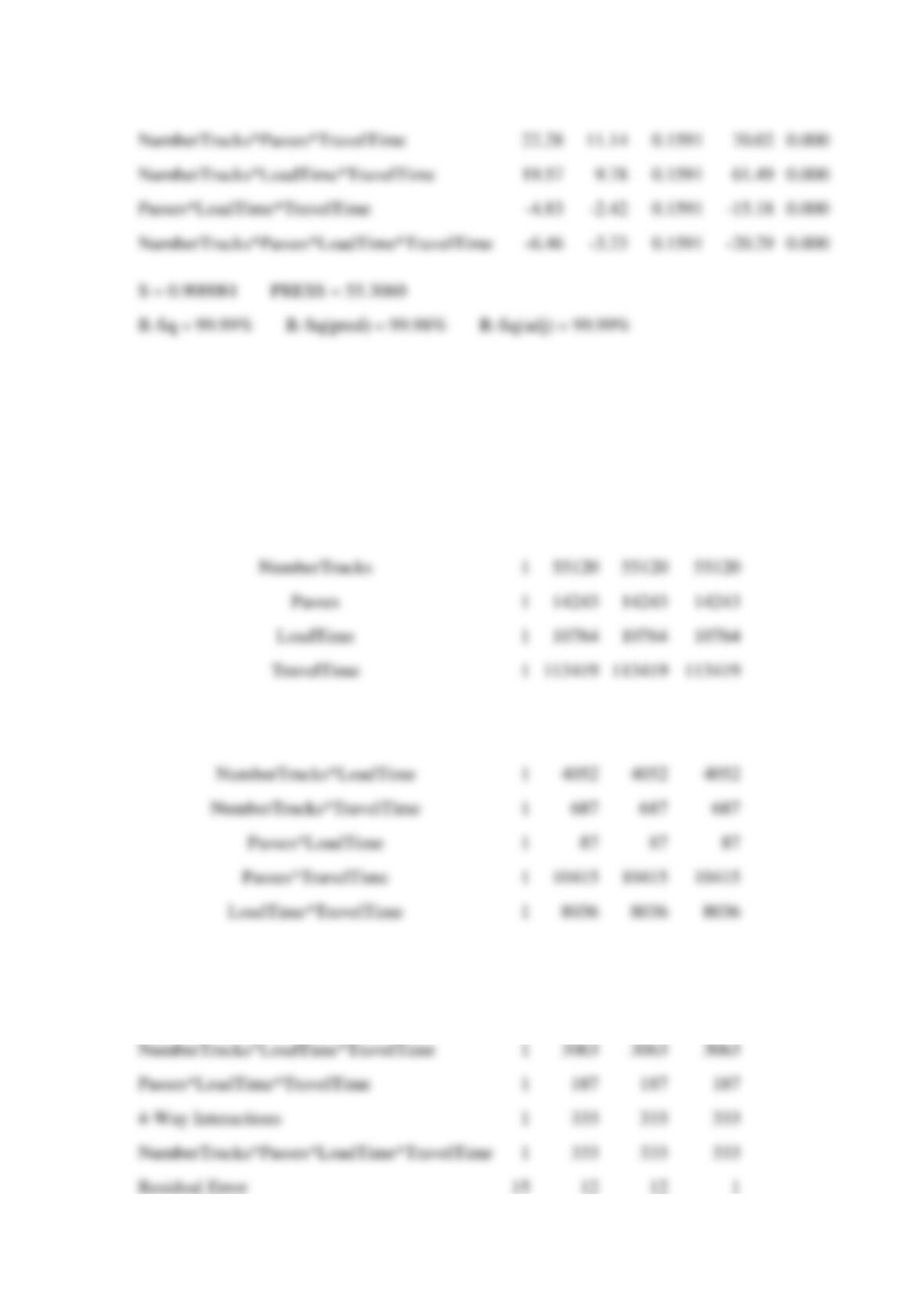
this experiment. Which two main effects are much greater than others?
(c) Conduct an ANOVA based on the two main effects, identified in part (b). Determine
sequential sums of squares for these effects.
SOLUTION
(a)
Estimated Effects and Coefficients for Production (coded units)
Term
Effect
Coef
SE Coef
T
P
Constant
138.43
0.1591
870.00
0.000
NumberTrucks
83.01
41.50
0.1591
260.84
0.000
Passes
-42.19
-21.10
0.1591
-132.59
0.000
LoadTime
-36.68
-18.34
0.1591
-115.27
0.000
TravelTime
-119.07
-59.53
0.1591
-374.16
0.000
NumberTrucks*Passes
-26.14
-13.07
0.1591
-82.15
0.000
NumberTrucks*LoadTime
-22.51
-11.25
0.1591
-70.72
0.000
NumberTrucks*TravelTime
-9.27
-4.63
0.1591
-29.13
0.000
Passes*LoadTime
1.65
0.1591
10.35
0.000
Passes*TravelTime
36.08
18.04
0.1591
113.38
0.000
Block
0.56
0.1591
0.003
NumberTrucks*Passes*LoadTime
5.57
2.78
0.1591
17.50
0.000
S = 0.900081 PRESS = 55.3060
R-Sq = 99.99% R-Sq(pred) = 99.98% R-Sq(adj) = 99.99%
Analysis of Variance for Production (coded units)
Source
DF
Seq SS
Adj SS
Adj MS
Blocks
1
10
10
10
Main Effects
4
193546
193546
48386
1
55120
55120
55120
1
14243
14243
14243
1
10764
10764
10764
1
113419
113419
2-Way Interactions
6
28745
28745
4791
NumberTrucks*Passes
1
5468
5468
5468
1
4052
4052
4052
1
687
687
687
1
87
87
87
1
10415
10415
10415
1
8036
8036
8036
3-Way Interactions
4
7470
7470
1867
NumberTrucks*Passes*LoadTime
1
248
248
248
NumberTrucks*Passes*TravelTime
1
3972
3972
3972
NumberTrucks*LoadTime*TravelTime
1
3063
3063
3063
Passes*LoadTime*TravelTime
1
187
187
187
4-Way Interactions
1
333
333
333
NumberTrucks*Passes*TravelTime
22.28
11.14
0.1591
70.02
0.000
NumberTrucks*LoadTime*TravelTime
19.57
9.78
0.1591
61.49
0.000
NumberTrucks*Passes*LoadTime*TravelTime
-6.46
-3.23
0.1591
-20.29
0.000
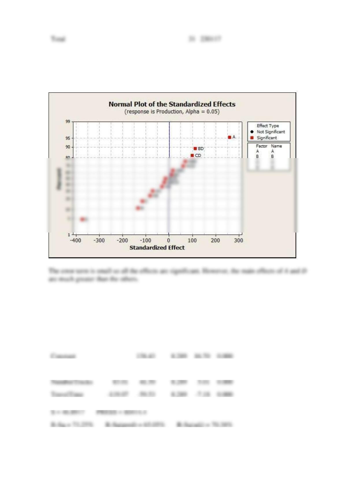
(b)
(c)
Estimated Effects and Coefficients for Production (coded units)
Term
Effect
Coef
SE Coef
T
P
Constant
8.289
16.70
0.000
Block
0.56
8.289
0.07
0.947
NumberTrucks
8.289
5.01
0.000
TravelTime
8.289
-7.18
0.000
S = 46.8917 PRESS = 80414.4
Total
230117