
14-21
14.5.5 An article in Journal of Construction Engineering and Management (“Analysis of Earth-Moving Systems Using
Discrete—Event Simulation,” 1995, Vol. 121(4), pp. 388–396) considered a replicated two-level factorial experiment
to study the factors most important to output in an earth-moving system. Handle the experiment as four replicates of a
24 factorial design with response equal to production rate (m3/h). The data are shown in the following table.
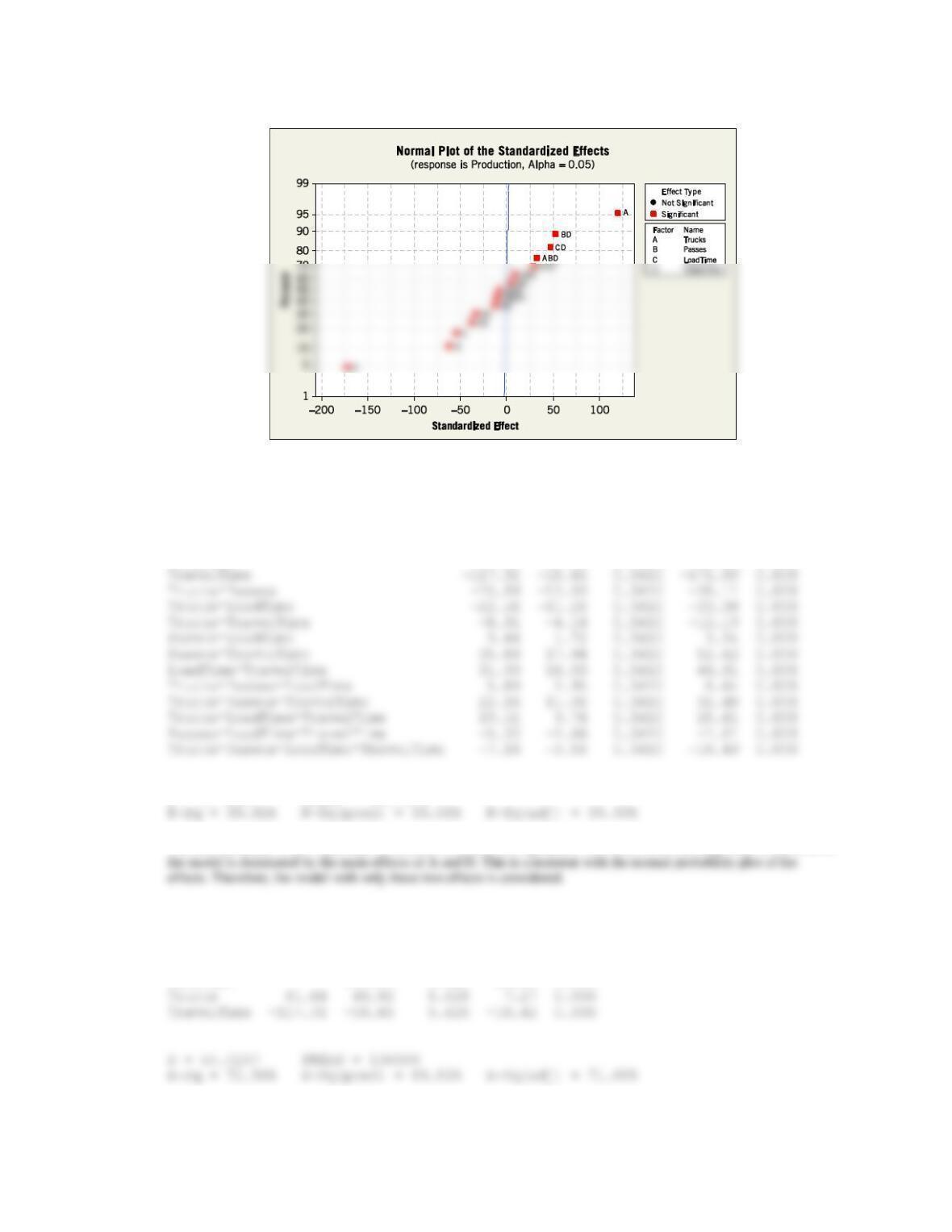
(a) Estimate the factor effects. Based on a normal probability plot of the effect estimates, identify a model for the data
from this experiment.
(b) Conduct an ANOVA based on the model identified in part (a). What are the conclusions?
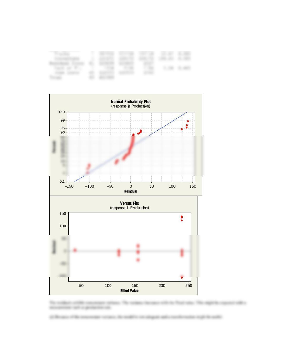
(c) Analyze the residuals and plot residuals versus the predicted production.
(d) Comment on model adequacy.
Level
−1
1
Number of trucks
2
6
Passes per load
4
7
Load pass time
12 s
22 s
Travel time
100 s
800 s
Row
Number of
Trucks
Passes per
Load
Load-pass
Time
Travel
Time
Production (m3/h)
1
2
3
4
1
−
−
−
−
179.6
179.8
176.3
173.1
2
+
−
−
−
373.1
375.9
372.4
361.1
3
−
+
−
−
153.2
153.6
150.8
148.6
4
+
+
−
−
226.1
220.0
225.7
218.5
5
−
−
+
−
156.9
155.4
154.2
152.2
6
+
−
+
−
242.0
233.5
242.3
233.6
7
−
+
+
−
122.7
119.6
120.9
118.6
8
+
+
+
−
135.7
130.9
135.5
131.6
9
−
−
−
+
44.2
44.0
43.5
43.6
10
+
−
−
+
124.2
123.3
122.8
121.6
11
−
+
−
+
42.0
42.4
42.5
41.0
12
+
+
−
+
116.3
117.3
115.6
114.7
13
−
−
+
+
42.1
42.6
42.8
42.9
14
+
−
+
+
119.1
119.5
116.9
117.2
15
−
+
+
+
39.6
39.7
39.5
39.2
16
+
+
+
+
107.0
105.3
104.2
103.0
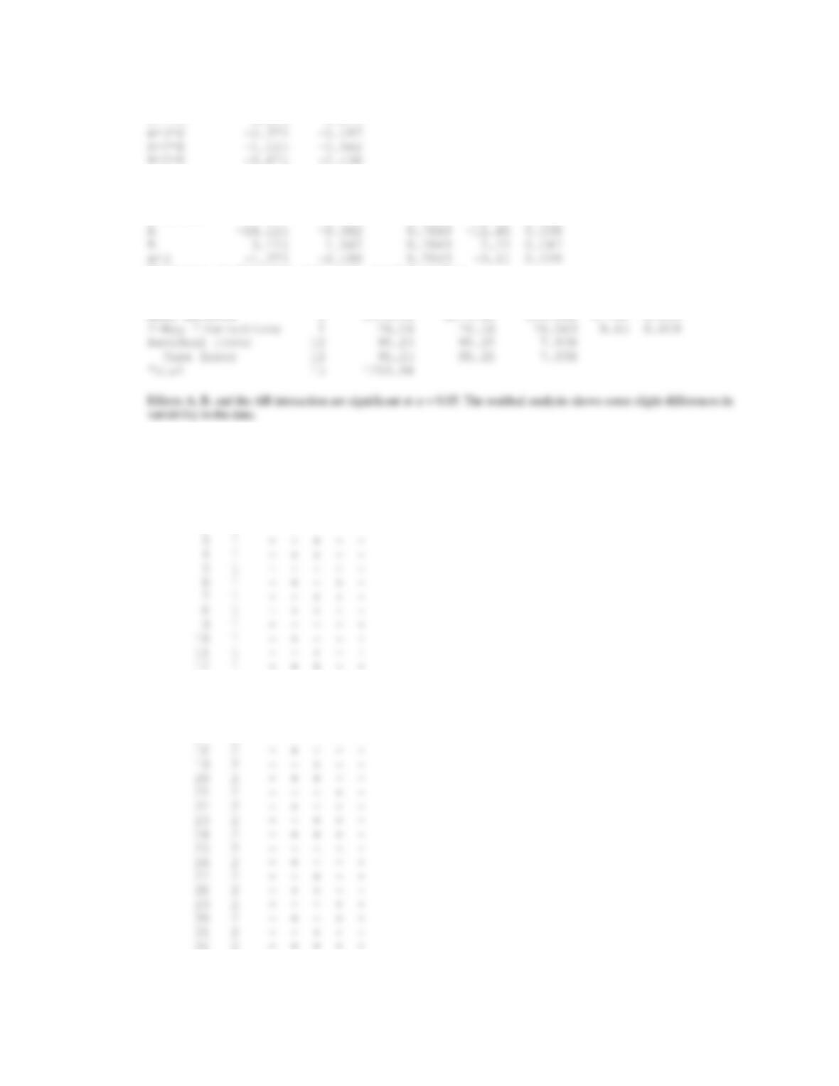
Applied Statistics and Probability for Engineers, 7th edition 2017
14-22
(a)
Estimated Effects and Coefficients for Production (coded units)
Term Effect Coef SE Coef T P
Constant 137.39 0.3410 402.87 0.000
Trucks 81.84 40.92 0.3410 119.98 0.000
Passes -42.20 -21.10 0.3410 -61.87 0.000
LoadTime -36.89 -18.45 0.3410 -54.09 0.000
S = 2.72827 PRESS = 635.173
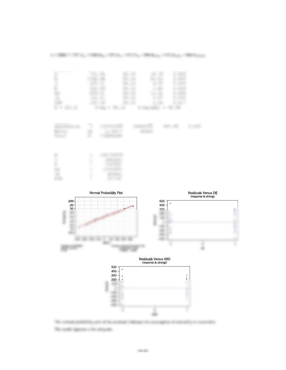
The error estimate in this experiment is small so all effects are significant. However, from the magnitude of the effects,
(b) An ANOVA with only the main effects of A and D follows.
Estimated Effects and Coefficients for Production (coded units)
Term Effect Coef SE Coef T P
Constant 137.39 5.628 24.41 0.000
Applied Statistics and Probability for Engineers, 7th edition 2017
14-23
Analysis of Variance for Production (coded units)
Source DF Seq SS Adj SS Adj MS F P
Main Effects 2 327330 327330 163665 80.75 0.000
(c)
Applied Statistics and Probability for Engineers, 7th edition 2017
14-24
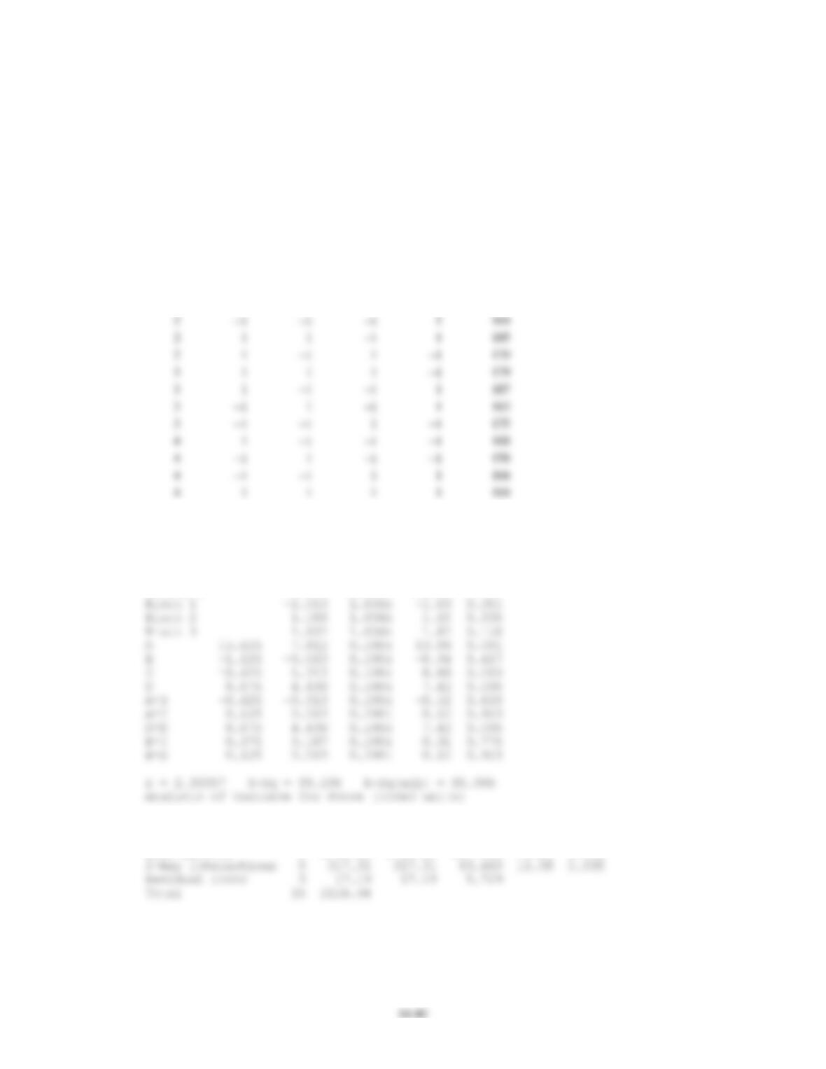
Section 14.6
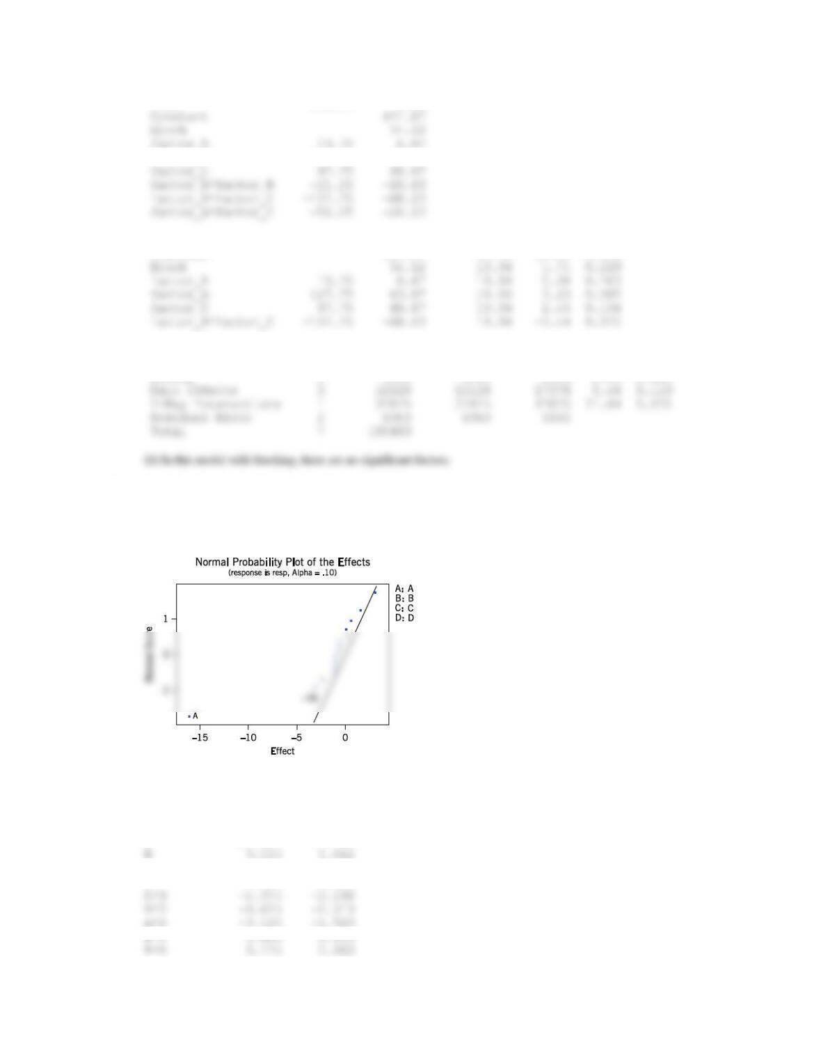
14.6.1 Consider the data from Exercise 14.5.2. Suppose that the data from the second replicate were not available. Analyze the
data from replicate I only and comment on your findings.
With only one replicate, the full factorial cannot be analyzed without using the three-way interaction for error.
Estimated Effects and Coefficients for resp (coded units)
Term Effect Coef SE Coef T P
Constant 411.88 34.13 12.07 0.053
A 13.75 6.88 34.12 0.20 0.873
B 127.75 63.87 34.12 1.87 0.312
C 97.75 48.88 34.13 1.43 0.388
14.6.2 The following data represent a single replicate of a 25 design that is used in an experiment to study the compressive
strength of concrete. The factors are mix (A), time (B), laboratory (C), temperature (D), and
drying time (E).
(1) = 700 e = 800
a = 900 ae = 1200
b = 3400 be = 3500
ab = 5500 abe = 6200
c = 600 ce = 600
ac = 1000 ace = 1200
bc = 3000 bce = 3006
abc = 5300 abce = 5500
d = 1000 de = 1900
ad = 1100 ade = 1500
bd = 3000 bde = 4000
abd = 6100 abde = 6500
cd = 800 cde = 1500
acd = 1100 acde = 2000
bcd = 3300 bcde = 3400
abcd = 6000 abcde = 6800
(a) Estimate the factor effects.
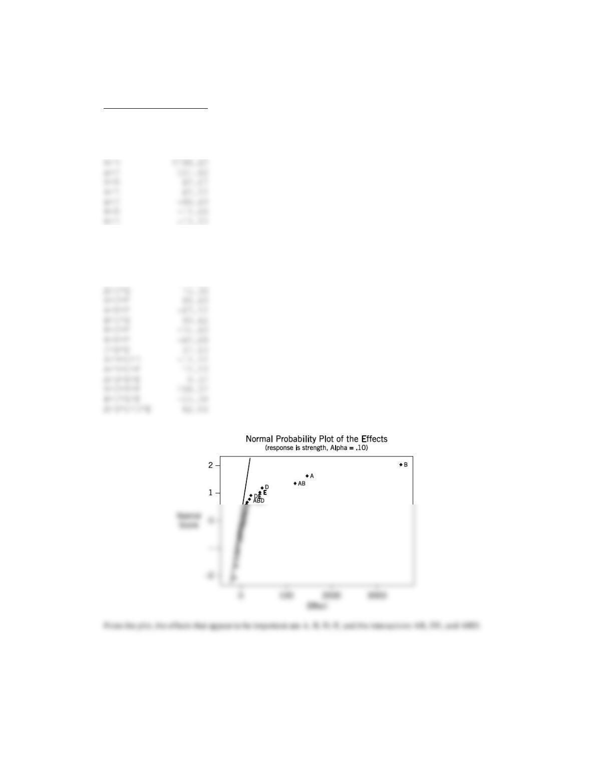
(b) Which effects appear important? Use a normal probability plot.
(c) If it is desirable to maximize the strength, in which direction would you adjust the process variables?
(d) Analyze the residuals from this experiment.
Applied Statistics and Probability for Engineers, 7th edition 2017
14-25
(a)
Estimated Effects and Coefficients for strength
Term Effect
A 1462.13
B 3537.87
C -137.12
D 474.62
E 425.38
C*D 112.13
C*E -62.13
D*E 224.62
A*B*C -62.88
A*B*D 200.38
A*B*E 49.63
(b)
Applied Statistics and Probability for Engineers, 7th edition 2017
(c) To maximize strength, the variables A, B, D, and E should be increased. Variable C is not significant. Thus, any
level of C is acceptable.
The regression equation is
Predictor Coef StDev T P
Constant 2887.69 39.10 73.86 0.000
Analysis of Variance
Source DF SS MS F P
Source DF Seq SS
A 1 17102476
(d)
14-27
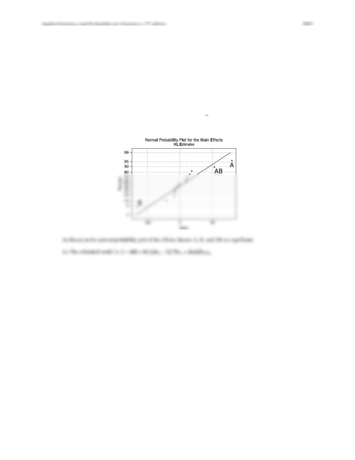
14.6.3 An experiment has run a single replicate of a 24 design and calculated the following factor effects:
A = 80.25 AB = 53.25 ABC = −2.95
B = −65.50 AC = 11.00 ABD = −8.00
C = −9.25 AD = 9.75 ACD = 10.25
D = −20.50 BC = 18.36 BCD = −7.95
BD = 15.10 ABCD = −6.25
CD = −1.25
(a) Construct a normal probability plot of the effects.
(b) Identify a tentative model, based on the plot of effects in part (a).
(c) Estimate the regression coefficients in this model, assuming that
=400y
.
(a)
14.6.4 An experiment described by M. G. Natrella in the National Bureau of Standards’ Handbook of Experimental
Statistics(1963, No. 91) involves flame-testing fabrics after applying fire-retardant treatments. The four factors
considered are type of fabric (A), type of fire-retardant treatment (B), laundering condition (C—the low level is no
laundering, the high level is after one laundering), and method of conducting the flame test (D). All factors are run at
two levels, and the response variable is the inches of fabric burned on a standard size test sample. The data are:
(1) = 42 d = 40
a = 31 ad = 30
b = 45 bd = 50
ab = 29 abd = 25
c = 39 cd = 40
ac = 28 acd = 25
bc = 46 bcd = 50
abc = 32 abcd = 23
(a) Estimate the effects and prepare a normal plot of the effects.
(b) Construct an analysis of variance table based on the model tentatively identified in part (a).
(c) Construct a normal probability plot of the residuals and comment on the results.
Applied Statistics and Probability for Engineers, 7th edition 2017
14-28
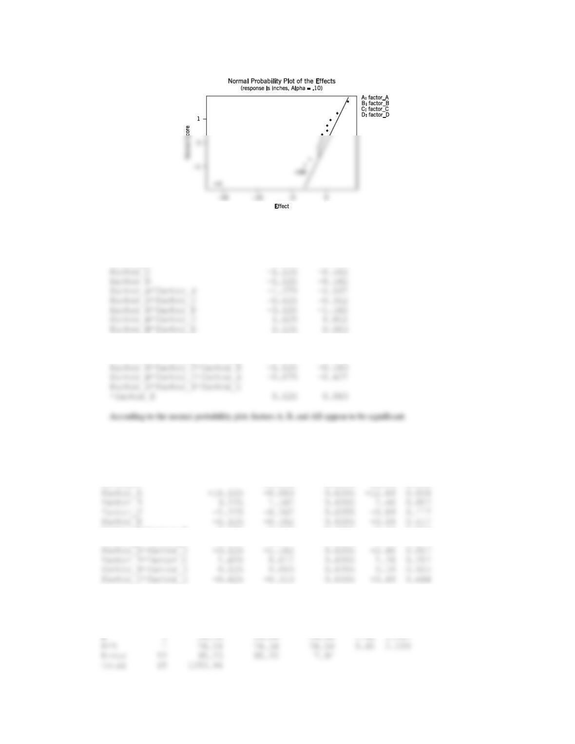
(a)
Estimated Effects and Coefficients for inches
Term Effect Coef
Constant 35.938
factor_A -16.125 -8.063
factor_B 3.125 1.562
factor_C*factor_D -0.625 -0.313
factor_A*factor_B*factor_C 0.625 0.313
factor_A*factor_B*factor_D -2.375 -1.188
Parts (b) and (c)
Remove the three- and four-factor interactions to generate the following analysis:
Term Effect Coef StDev Coef T P
Constant 35.938 0.6355 56.55 0.000
factor_A*factor_B -4.375 -2.187 0.6355 -3.44 0.018
factor_A*factor_C -0.625 -0.312 0.6355 -0.49 0.644
Analysis of Variance for resp, using Adjusted SS for Tests
Source DF Seq SS Adj SS Adj MS F P
A 1 1040.06 1040.06 1040.06 131.03 0.000
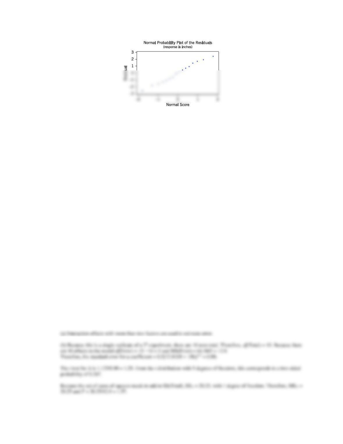
Applied Statistics and Probability for Engineers, 7th edition 2017
14-29
14.6.5 Consider the following computer output for one replicate of a 24 factorial experiment.
(a) What effects are used to estimate error?
(b) Calculate the entries marked with “?” in the output.
Estimated Effects and Coefficients
Term Effect Coef SE Coef t P
Constant 35.250 ? 39.26 0.000
A 2.250 ? ? ? ?
B 24.750 12.375 ? 13.78 0.000
C 1.000 0.500 ? 0.56 0.602
D 10.750 5.375 ? 5.99 0.002
A*B −10.500 −5.250 ? −5.85 0.002
A*C 4.250 2.125 ? 2.37 0.064
A*D −5.000 −2.500 ? −2.78 0.039
B*C 5.250 2.625 ? 2.92 0.033
B*D 4.000 2.000 ? 2.23 0.076
C*D −0.750 −0.375 ? −0.42 0.694
S = 3.59166
Analysis of Variance
Source DF SS MS F P
A ? ? ? ? 0.266
B 1 2450.25 2450.25 189.94 0.000
C 1 4.00 4.00 0.31 0.602
D 1 462.25 462.25 35.83 0.002
AB 1 441.00 441.00 34.19 0.002
AC 1 72.25 72.25 5.60 0.064
AD 1 100.00 100.00 7.75 0.039
BC 1 110.25 110.25 8.55 0.033
BD 1 64.00 64.00 4.96 0.076
CD 1 2.25 2.25 0.17 0.694
Residual Error ? 64.50 ?
Total ? 3791.00
Applied Statistics and Probability for Engineers, 7th edition 2017
14-30
Estimated Effects and Coefficients
Term Effect Coef SE Coef t P
Constant 35.250 0.90 39.26 0.000
A 2.250 1.125 0.90 1.25 0.267
B 24.750 12.375 0.90 13.78 0.000
A*C 4.250 2.125 0.90 2.37 0.064
A*D -5.000 -2.500 0.90 -2.78 0.039
Analysis of Variance
Source DF SS MS F P
A 1 20.25 20.25 1.57 0.266
D 1 462.25 462.25 35.83 0.002
14.6.6 An article in Bioresource Technology (“Influence of Vegetable Oils Fatty-Acid Composition on Biodiesel
Optimization,” (2011, Vol. 102(2), pp. 1059–1065)] described an experiment to analyze the influence of the fatty-acid
composition on biodiesel. Factors were the concentration of catalyst, amount of methanol, reaction temperature and
time, and the design included three center points. Maize oil methyl ester (MME) was recorded as the response. Data
follow.
Run
Temperature
(°C)
Time (min)
Catalyst (wt.%)
Methanol to oil
molar ratio
MME (wt. %)
1
45
40
0.8
5.4
88.30
2
25
40
1.2
5.4
90.50
3
45
10
0.8
4.2
77.96
4
25
10
1.2
5.4
85.59
5
45
40
1.2
5.4
97.14
6
45
10
1.2
4.2
90.64
7
45
40
1.2
4.2
89.86
8
25
40
0.8
4.2
82.35
9
25
10
0.8
5.4
80.31
10
25
40
0.8
5.4
85.51
11
25
10
0.8
4.2
76.21
12
45
40
0.8
4.2
86.86
13
25
10
1.2
4.2
86.35
14
45
10
0.8
5.4
84.58
15
25
40
1.2
4.2
89.37
16
45
10
1.2
5.4
90.51
17
35
25
1
4.8
91.40
18
35
25
1
4.8
91.96
19
35
25
1
4.8
91.07
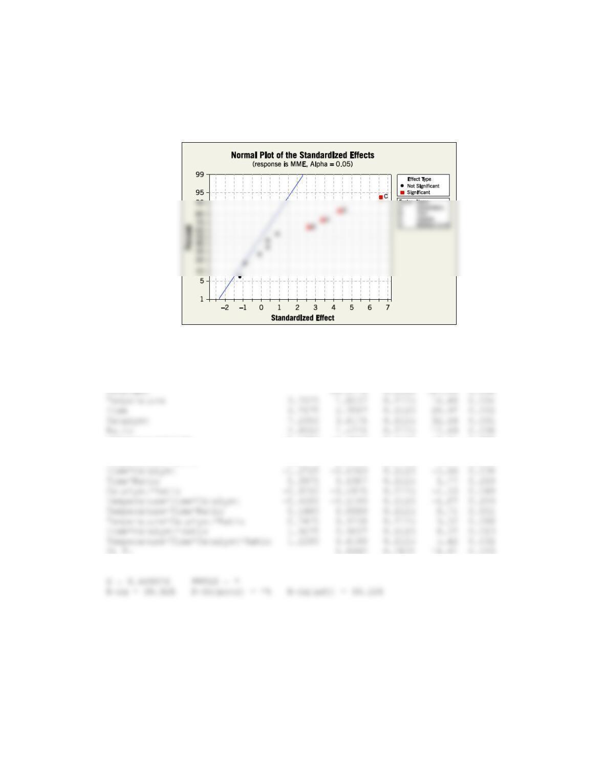
(a) Identify the important effects from a normal probability plot.
Applied Statistics and Probability for Engineers, 7th edition 2017
14-31
(b) Compare the results in the previous part with results that use an error term based on the center points.
(c) Test for curvature.
(d) Analyze the residuals from the model.
(a) Identify the important factor with a normal probability plot based on the corner points.
(b) Compare the results in the previous part with results that use an error term based on the center points.
Estimated Effects and Coefficients for MME (coded units)
Term Effect Coef SE Coef T P
Temperature*Time -0.1000 -0.0500 0.1125 -0.44 0.700
Temperature*Catalyst 0.3775 0.1888 0.1125 1.68 0.235
Temperature*Ratio 0.9475 0.4737 0.1125 4.21 0.052
Applied Statistics and Probability for Engineers, 7th edition 2017
14-32
Analysis of Variance for MME (coded units)
Source DF Seq SS Adj SS Adj MS F
Main Effects 4 385.986 385.986 96.497 476.68
Temperature 1 54.982 54.982 54.982 271.61
Time*Catalyst 1 6.477 6.477 6.477 32.00
Time*Ratio 1 0.632 0.632 0.632 3.12
Catalyst*Ratio 1 3.803 3.803 3.803 18.78
3-Way Interactions 4 17.904 17.904 4.476 22.11
Source P
Main Effects 0.002
Temperature 0.004
Temperature*Time 0.700
Temperature*Catalyst 0.235
Temperature*Ratio 0.052
Applied Statistics and Probability for Engineers, 7th edition 2017
14-33
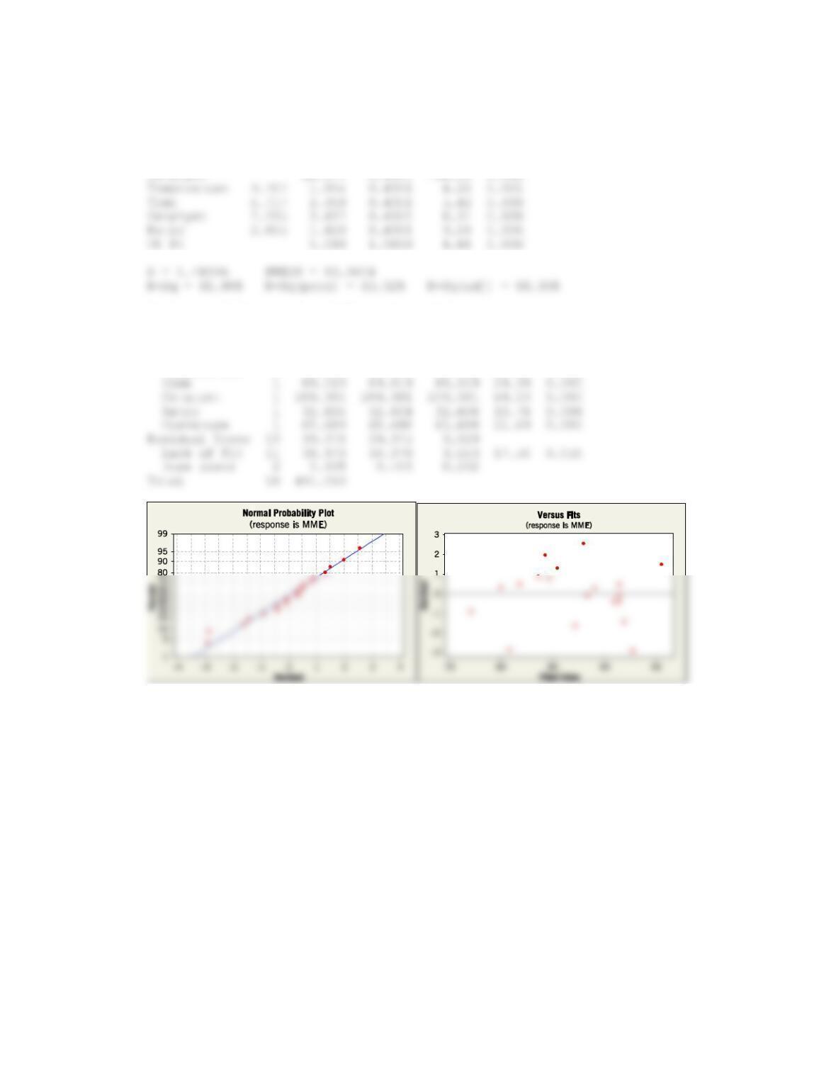
(d) A model with only the four main effects and the center point term is used to generate residuals.
Estimated Effects and Coefficients for MME (coded units)
Term Effect Coef SE Coef T P
Analysis of Variance for MME (coded units)
Source DF Seq SS Adj SS Adj MS F P
Main Effects 4 385.986 385.986 96.497 31.86 0.000
Temperature 1 54.982 54.982 54.982 18.15 0.001
There are no obvious departures from assumptions seen in these plots.

Applied Statistics and Probability for Engineers, 7th edition 2017
14-34
14.6.7 An article in Analytica Chimica Acta [“Design–of-Experiment Optimization of Exhaled Breath Condensate Analysis
Using a Miniature Differential Mobility Spectrometer (DMS)” (2008, Vol. 628(2), pp. 155–161)] examined four
parameters that affect the sensitivity and detection of the analytical instruments used to measure clinical samples. They
optimized the sensor function using exhaled breath condensate (EBC) samples spiked
with acetone, a known clinical biomarker in breath. The following table shows the results for a single replicate of a 24
factorial experiment for one of the outputs, the average amplitude of acetone peak over three repetitions.
Configuration
A
B
C
D
y
1
+
+
+
+
0.12
2
+
+
+
−
0.1193
3
+
+
−
+
0.1196
4
+
+
−
−
0.1192
5
+
−
+
+
0.1186
6
+
−
+
−
0.1188
7
+
−
−
+
0.1191
8
+
−
−
−
0.1186
9
−
+
+
+
0.121
10
−
+
+
−
0.1195
11
−
+
−
+
0.1196
12
−
+
−
−
0.1191
13
−
−
+
+
0.1192
14
−
−
+
−
0.1194
15
−
−
−
+
0.1188
16
−
−
−
−
0.1188
The factors and levels are shown in the following table.
A RF voltage of the DMS sensor (1200 or 1400 V)
B Nitrogen carrier gas flow rate (250 or 500 mL min−1)
C Solid phase micro extraction (SPME) filter type (polyacrylate or PDMS–DVB)
D GC cooling profile (cryogenic and noncryogenic)
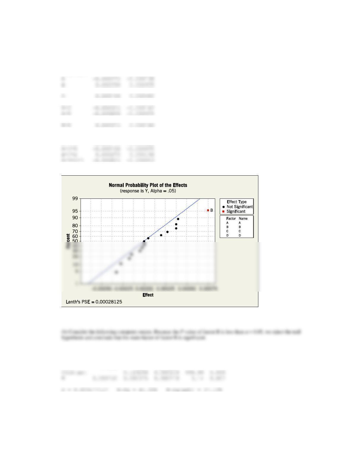
(a) Estimate the factor effects and use a normal probability plot of the effects. Identify which effects appear to be large,
and identify a model for the data from this experiment.
(b) Conduct an ANOVA based on the model identified in part (a). What are your conclusions?
(c) Analyze the residuals from this experiment. Are there any problems with model adequacy?
(d) Project the design in this problem into a 2rdesign for r < 4 in the important factors. Sketch the design and show the
average and range of yields at each run. Does this sketch aid in data representation?
Applied Statistics and Probability for Engineers, 7th edition 2017
14-35
(a)
Factorial Fit: Y versus A, B, C, D
Estimated Effects and Coefficients for Y (coded units)
Term Effect Coef
Constant 0.119288
C 0.000375 0.000188
A*B 0.000000 0.000000
B*C 0.000200 0.000100
C*D 0.000050 0.000025
A*B*C 0.000000 0.000000
A*B*D -0.000175 -0.000088
A*B*C*D -0.000025 -0.000013
The effect of factor B is large, so this factor is included in the model.
Factorial Fit: Y versus B
Estimated Effects and Coefficients for Y (coded units)
Term Effect Coef SE Coef T P
Applied Statistics and Probability for Engineers, 7th edition 2017
14-36
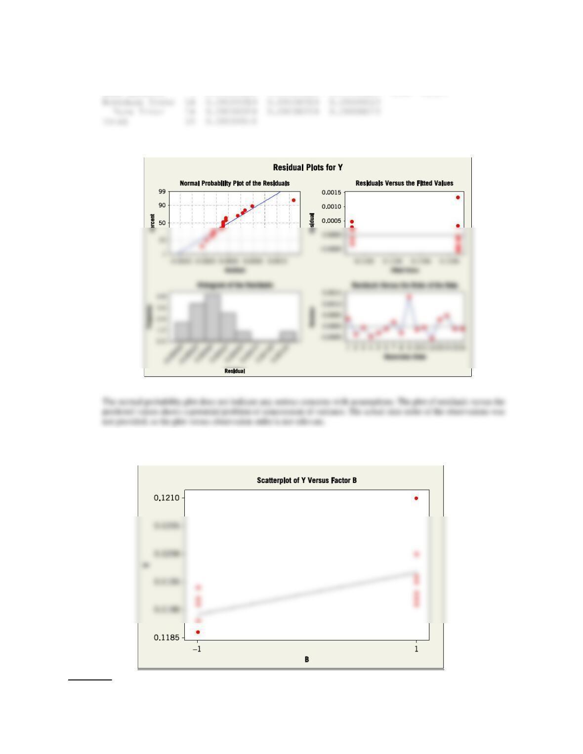
Analysis of Variance for Y (coded units)
Source DF Seq SS Adj SS Adj MS F P
Main Effects 1 0.00000225 0.00000225 0.00000225 9.88 0.007
(c)
(d) Only one main factor B is significant. The design is reduced to eight replicates of an experiment with a single factor
with two levels. The scatter plot of Y and factor B indicates that an increase to factor B increases the response.
Section 14.7
Applied Statistics and Probability for Engineers, 7th edition 2017
14-37
14.7.1 Consider a 22 factorial experiment with four center points. The data are (1) = 21, a = 125, b = 154, ab = 352, and the
responses at the center point are 92, 130, 98, 152. Compute an ANOVA with the sum of squares for curvature and
conduct an F-test for curvature. Use
= 0.05.
Only main effects are significant. Interaction effects and curvature are not significant at
= 0.05.
Analysis of Variance for Response (coded units)
Source DF Seq SS Adj SS Adj MS F P
Main Effects 2 55201 55201 27600.5 34.85 0.008
14.7.2 Consider the experiment in Exercise 14.6.2. Suppose that a center point with five replicates is added to the factorial
runs and the responses are 2800, 5600, 4500, 5400, 3600. Compute an ANOVA with the sum of squares for curvature
and conduct an F-test for curvature. Use
= 0.05.
Only curvature is significant at
= 0.05.
Analysis of Variance for Strength (coded units)
Source DF Seq SS Adj SS Adj MS F P
Main Effects 5 120635081 120635081 24127016 17.09 0.008
Section 14.8
14.8.1 Consider the data from the first replicate of Exercise 14.5.2.
(a) Suppose that these observations could not all be run under the same conditions. Set up a design to run these
Observations in two blocks of four observations each with ABC confounded.
(b) Analyze the data.
(a)
BLOCK
A
B
C
y
1
−1
−1
−1
221
1
1
1
−1
552
1
1
−1
1
406
−1
2
1
−1
−1
325
2
−1
1
−1
354
2
−1
−1
1
440
Applied Statistics and Probability for Engineers, 7th edition 2017
14-38
Term Effect Coef
factor_A 13.75 6.87
factor_B 127.75 63.87
Term Effect Coef StDev Coef T P
Constant 411.87 19.94 20.65 0.002
Analysis of Variance for life
Source DF Seq SS Adj SS Adj MS F P
Blocks 1 9316 9316 9316 2.93 0.229
14.8.2 Consider the data from Exercise 14.6.4.
(a) Construct the design that would have been used to run this experiment in two blocks of eight runs each.
(b) Analyze the data and draw conclusions.
Factor A and interaction AB are significant. Factor B is included in the model to make the model hierarchical.
Term Effect Coef
Constant 35.938
BLOCK -0.063
A -16.125 -8.062
C -1.125 -0.562
D -1.125 -0.562
Applied Statistics and Probability for Engineers, 7th edition 2017
14-39
C*D -0.625 -0.312
A*B*C 0.625 0.312
B*C*D -0.875 -0.438
Estimated Effects and Coefficients for resp (coded units)
Term Effect Coef SE Coef T P
Constant 35.938 0.7043 51.02 0.000
Analysis of Variance for resp (coded units)
Source DF Seq SS Adj SS Adj MS F P
14.8.3 Construct a 25design in two blocks. Select the ABCDE interaction to be confounded with blocks.
25 Design in 2 Blocks with ABCDE confounded with blocks.
Run Block A B C D E
1 1 – – – – –
2 1 + + – – –
13 1 – – – + +
14 1 + + – + +
15 1 + – + + +
16 1 – + + + +
17 2 + – – – –
Applied Statistics and Probability for Engineers, 7th edition 2017
14.8.4 Consider the data from the first replicate of Exercise 14.5.1, assuming that four blocks are required. Confound ABD and
ABC (and consequently CD) with blocks.
(a) Construct a design with four blocks of four observations each.
(b) Analyze the data.
(a) The design with four blocks
Blocks
A
B
C
D
Score
1
−1
1
1
1
170
1
1
1
−1
−1
166
1
−1
−1
−1
−1
159
1
1
−1
1
1
197
2
−1
1
1
−1
173
2
−1
−1
−1
1
164
2
1
1
−1
1
185
2
1
−1
1
−1
179
3
1
1
1
−1
179
3
1
−1
−1
1
187
3
−1
1
−1
1
163
3
−1
−1
1
−1
175
4
1
−1
−1
−1
168
4
−1
1
−1
−1
158
4
−1
−1
1
1
168
4
1
1
1
1
194
(b)
Estimated Effects and Coefficients for Score (coded units)
Term Effect Coef SE Coef T P
Constant 174.063 0.5984 290.88 0.000
Source DF Seq SS Adj SS Adj MS F P
Blocks 3 42.19 42.19 14.063 2.45 0.240
Main Effects 4 1748.25 1748.25 437.063 76.29 0.002