Analysis of Variance for Production (coded units)
Source
DF
Seq SS
Adj SS
Adj MS
F
P
Blocks
1
10
10
10
0.00
0.947
TravelTime
1
113419
113419
113419
51.58
0.000
Residual Error
28
61567
61567
2199
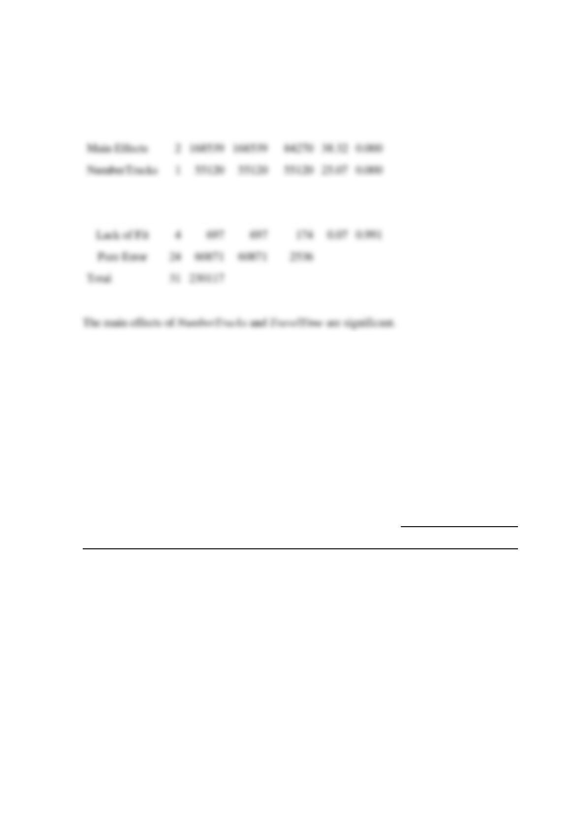
Lack of Fit
4
697
697
174
0.07
0.991
24
60871
60871
2536
Total
31
230117
Reserve Problems Chapter 14 Section 8 Problem 4
An article in Journal of Hazardous Materials [“Biosorption of Reactive Dye Using Acid-Treated
Rice Husk: Factorial Design Analysis” (2007, Vol. 142(1), pp. 397–403)] described an
experiment using biosorption to remove red color from water. A
4
2
full factorial design was
used to study the effect of factors pH, temperature, adsorbent dosage, and initial concentration of
the dye. Consider columns 1 and 2 under the response Removal Efficiency (%) to define the
blocks in this design
Run
pH
Dosage
(g/L)
Concentration
(mg/L)
Temperature
(°C)
Removal Efficiency
(%)
1
2
1
2
5
50
20
89.36
95.78
2
7
5
50
20
53.67
52.02
3
2
50
50
20
86.97
93.76
4
7
50
50
20
72.39
80.55
5
2
5
250
20
68.46
64.99
6
7
5
250
20
32.44
28.44
7
2
50
250
20
93.19
93.69
8
7
50
250
20
88.17
91.41
9
2
5
50
40
97.25
95.41
Main Effects
2
168539
168539
84270
38.32
0.000
NumberTrucks
1
55120
55120
55120
25.07
0.000
10
7
5
50
40
76.42
56.51
11
2
50
50
40
76.24
90.83
12
7
50
50
40
79.54
73.21
13
2
5
250
40
84.31
82.84
14
7
5
250
40
53.32
44.96
15
2
50
250
40
94.77
96.53
16
7
50
250
40
89.32
90.75
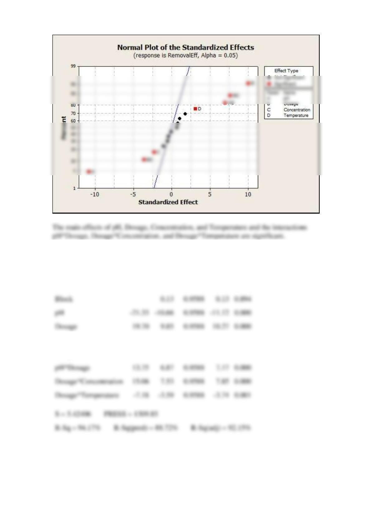
(a) Estimate the factor effects. Based on a normal probability plot of the effect estimates,
identify a model for the data from this experiment. Which main effects and interactions are
significant?
(b) Conduct an ANOVA based on the model that uses only significant effects and interactions
determined in part (a). Find the sequential sums of squares for this effects and interactions.
SOLUTION
(a)
Estimated Effects and Coefficients for Removal Efficiency (coded units)
Term
Effect
Coef
SE Coef
T
P
Constant
77.11
0.9812
78.59
0.000
Concentration
-4.52
-2.26
0.9812
-2.30
0.036
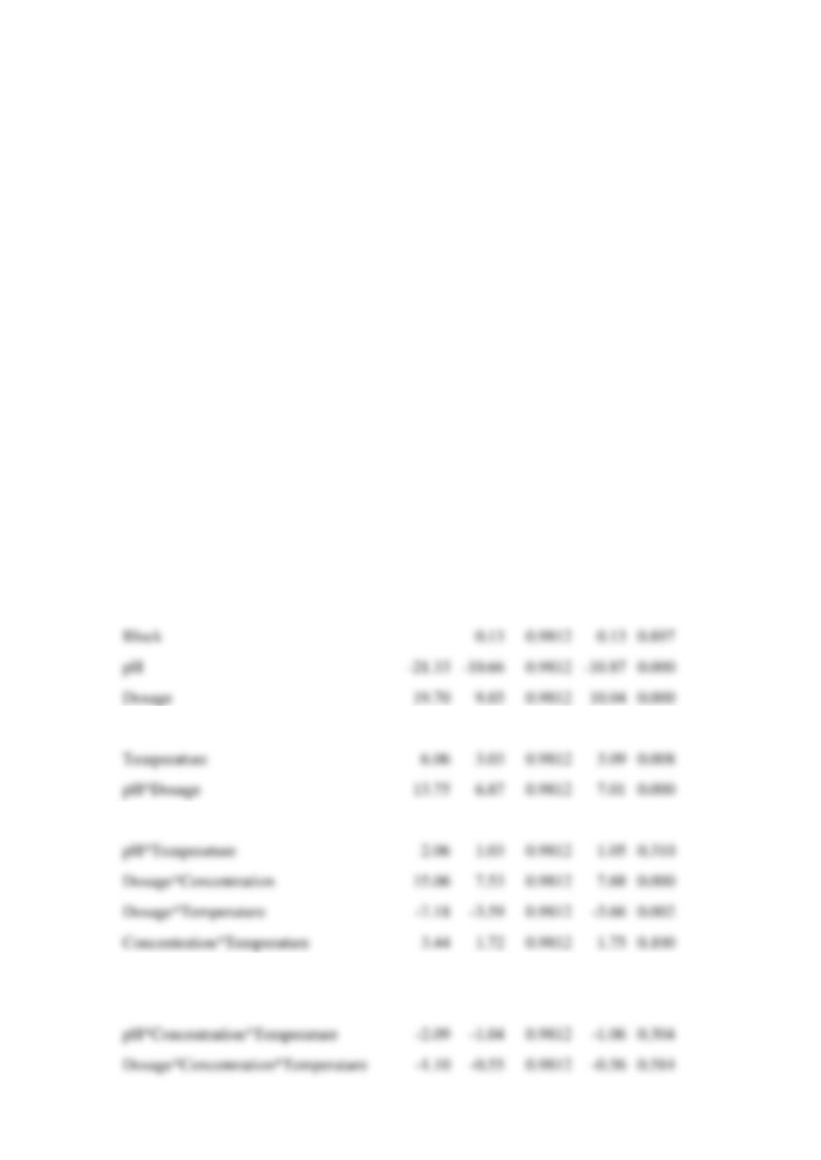
Temperature
6.06
3.03
0.9812
3.09
0.008
pH*Dosage
13.75
6.87
0.9812
7.01
0.000
pH*Concentration
1.33
0.67
0.9812
0.68
0.507
pH*Temperature
2.06
1.03
0.9812
1.05
0.310
Dosage*Concentration
15.06
7.53
0.9812
7.68
0.000
Dosage*Temperature
-7.18
-3.59
0.9812
-3.66
0.002
Concentration*Temperature
3.44
1.72
0.9812
1.75
0.100
pH*Dosage*Concentration
1.61
0.81
0.9812
0.82
0.423
pH*Dosage*Temperature
-0.87
-0.43
0.9812
-0.44
0.665
Block
0.13
0.9812
0.13
0.897
pH
-21.33
-10.66
0.9812
-10.87
0.000
Dosage
19.70
9.85
0.9812
10.04
0.000
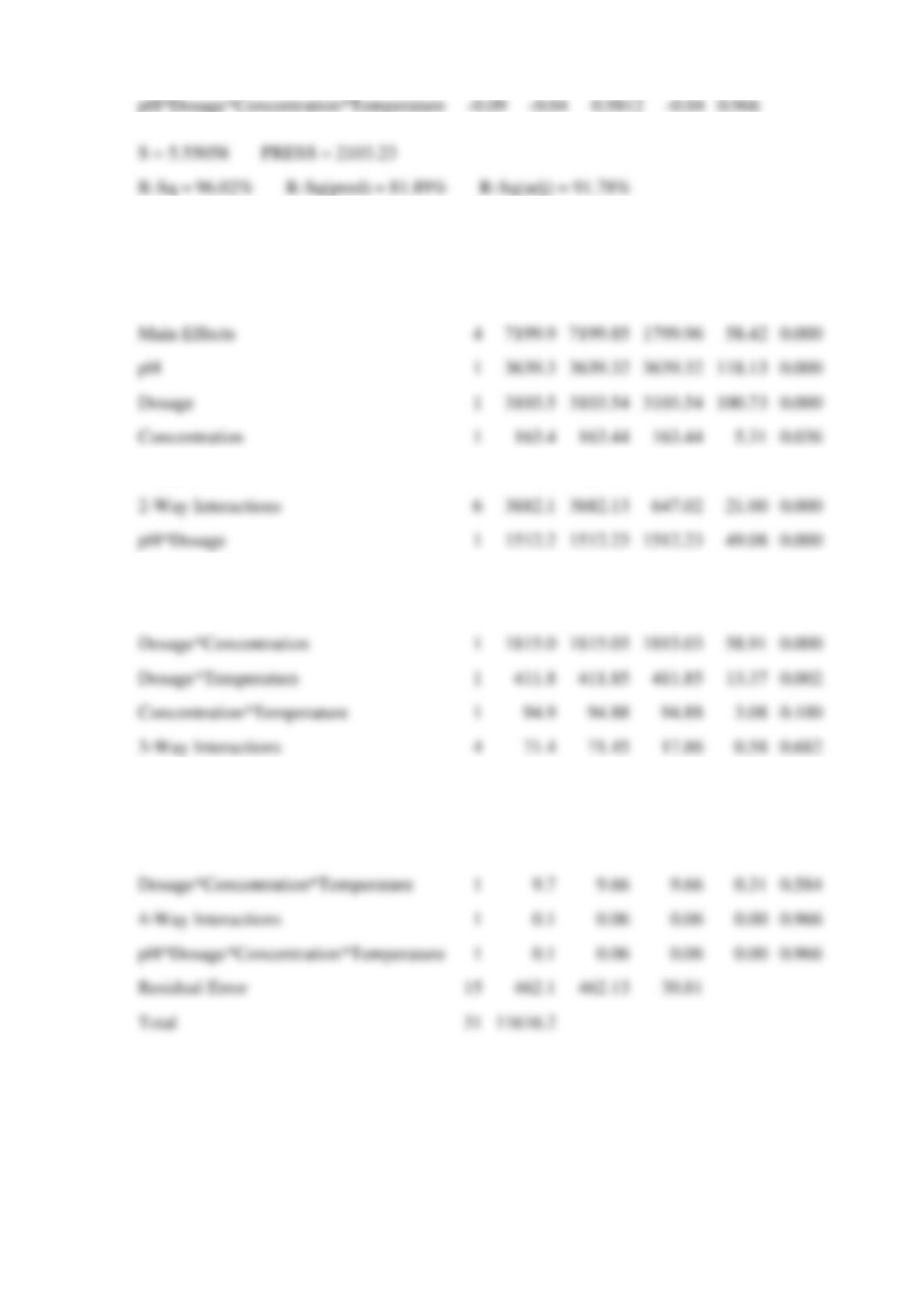
S = 5.55058 PRESS = 2103.23
R-Sq = 96.02% R-Sq(pred) = 81.89% R-Sq(adj) = 91.78%
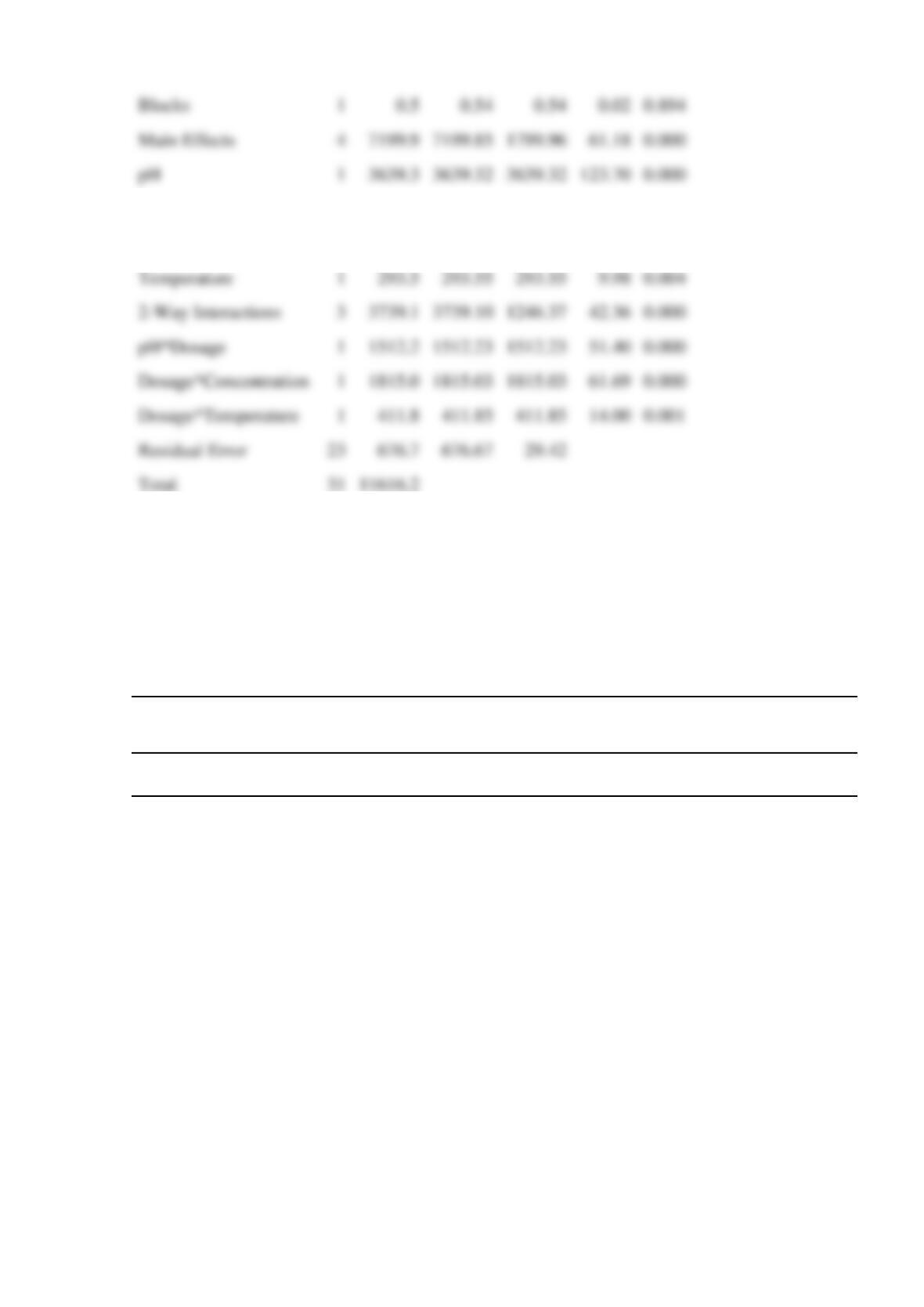
Analysis of Variance for Removal Efficiency (coded units)
Source
DF
Seq SS
Adj SS
Adj MS
F
P
Blocks
1
0.5
0.54
0.54
0.02
0.897
Main Effects
4
7199.9
7199.85
1799.96
58.42
0.000
pH
1
3639.3
3639.32
3639.32
118.13
0.000
Dosage
1
3103.5
3103.54
3103.54
100.73
0.000
Concentration
1
163.4
163.44
163.44
5.31
0.036
Temperature
1
293.5
293.55
293.55
9.53
0.008
2-Way Interactions
6
3882.1
3882.13
647.02
21.00
0.000
pH*Dosage
1
1512.2
1512.23
1512.23
49.08
0.000
pH*Concentration
1
14.2
14.20
14.20
0.46
0.507
pH*Temperature
1
33.9
33.95
33.95
1.10
0.310
Dosage*Temperature
1
411.8
411.85
411.85
13.37
0.002
Concentration*Temperature
1
94.9
94.88
94.88
3.08
0.100
3-Way Interactions
4
71.4
71.45
17.86
0.58
0.682
pH*Dosage*Concentration
1
20.9
20.87
20.87
0.68
0.423
pH*Dosage*Temperature
1
6.0
6.02
6.02
0.20
0.665
pH*Concentration*Temperature
1
34.9
34.90
34.90
1.13
0.304
Dosage*Concentration*Temperature
1
9.7
9.66
9.66
0.31
0.584
4-Way Interactions
1
0.1
0.06
0.06
0.00
0.966
pH*Dosage*Concentration*Temperature
1
0.1
0.06
0.06
0.00
0.966
Residual Error
462.1
462.13
30.81
Total
11616.2
pH*Dosage*Concentration*Temperature
-0.09
-0.04
-0.04
0.966
(b)
Estimated Effects and Coefficients for Removal Efficiency (coded units)
Term
Effect
Coef
SE Coef
T
P
Constant
77.11
0.9588
78.59
0.000
Block
0.13
0.9588
0.13
0.894
pH
-21.33
-10.66
0.9588
-11.12
0.000
Dosage
19.70
9.85
0.9588
10.27
0.000
Concentration
-4.52
-2.26
0.9588
-2.36
0.027
Temperature
6.06
3.03
0.9588
3.16
0.004
pH*Dosage
13.75
6.87
0.9588
7.17
0.000
Dosage*Concentration
15.06
7.53
0.9588
7.85
0.000
Dosage*Temperature
-7.18
-3.59
0.9588
-3.74
0.001
S = 5.42406 PRESS = 1309.85
R-Sq = 94.17% R-Sq(pred) = 88.72% R-Sq(adj) = 92.15%
Analysis of Variance for Removal Efficiency (coded units)
Source
DF
Seq SS
Adj SS
Adj MS
F
P
Dosage
1
3103.5
3103.54
3103.54
105.49
0.000
Concentration
1
163.4
163.44
163.44
5.56
0.027
Temperature
1
293.5
293.55
293.55
9.98
0.004
2-Way Interactions
3
3739.1
3739.10
1246.37
42.36
0.000
pH*Dosage
1
1512.2
1512.23
1512.23
51.40
0.000
Dosage*Concentration
1
1815.0
1815.03
1815.03
61.69
0.000
Dosage*Temperature
1
411.8
411.85
411.85
14.00
0.001
Residual Error
676.7
676.67
29.42
Total
11616.2
Reserve Problems Chapter 14 Section 10 Problem 1
A
84
2−
fractional factorial design is used to identify sources of Pu contamination in the
radioactivity material analysis of dried shellfish. The data are shown in the following table. No
contamination occurred at runs 1, 4, and 9. The factors and levels are shown in the following
table.
84
2−
Glassware
Reagent
Sample
Prep
Tracer
Dissolution
Hood
Chemistry
Ashing
mBq
Run
1
x
2
x
3
x
4
x
5
x
6
x
7
x
8
x
y
1
-1
-1
-1
-1
-1
-1
-1
-1
0
2
+1
-1
-1
-1
-1
+1
+1
+1
3.31
3
-1
+1
-1
-1
+1
-1
+1
+1
0.0373
4
+1
+1
-1
-1
+1
+1
-1
-1
0
5
-1
-1
+1
-1
+1
+1
+1
-1
0.0649
6
+1
-1
+1
-1
+1
-1
-1
+1
0.133
7
-1
+1
+1
-1
-1
+1
-1
+1
0.0461
8
+1
+1
+1
-1
-1
-1
+1
-1
0.0297
9
-1
-1
-1
+1
+1
+1
-1
+1
0
10
+1
-1
-1
+1
+1
-1
+1
-1
0.287
11
-1
+1
-1
+1
-1
+1
+1
-1
0.133
12
+1
+1
-1
+1
-1
-1
-1
+1
0.0476
Blocks
1
0.02
0.894
Main Effects
4
7199.9
7199.85
1799.96
61.18
0.000
pH
1
3639.3
3639.32
3639.32
123.70
0.000

13
-1
-1
+1
+1
-1
-1
+1
+1
0.133
14
+1
-1
+1
+1
-1
+1
-1
-1
5.75
15
-1
+1
+1
+1
+1
-1
-1
-1
0.0153
16
+1
+1
+1
+1
+1
+1
+1
+1
2.47
Factor
–1
+1
Glassware
Distilled water
Soap, acid, stored
Reagent
New
Old
Sample prep
Coprecipitation
Electrodeposition
Tracer
Stock
Fresh
Dissolution
Without
With
Hood
B
A
Chemistry
Without
With
Ashing
Without
With
(a) Generators and complete defining relation for this design are _______.
(b) Estimate the main effects. Indicate the factors with the largest and the smallest effect and
enter your estimation.
(c) From the effects table and the normal probability plot choose four less important factors for
using those terms to estimate errors.
(d) Analyze the design identified in (c) and its important factors.
Determine the adjusted error mean square.
Determine the value of test statistic for main effects.
Determine the value of test statistic for 2-way interactions.
SOLUTION
Alias Structure (up to order 4)
I ABCG ABDH ABEF ACDF ACEH ADEG AFGH BCDE BCFH
BDFG BEGH CDGH CEFG DEFH
= = = = = = = = =
= = = = =
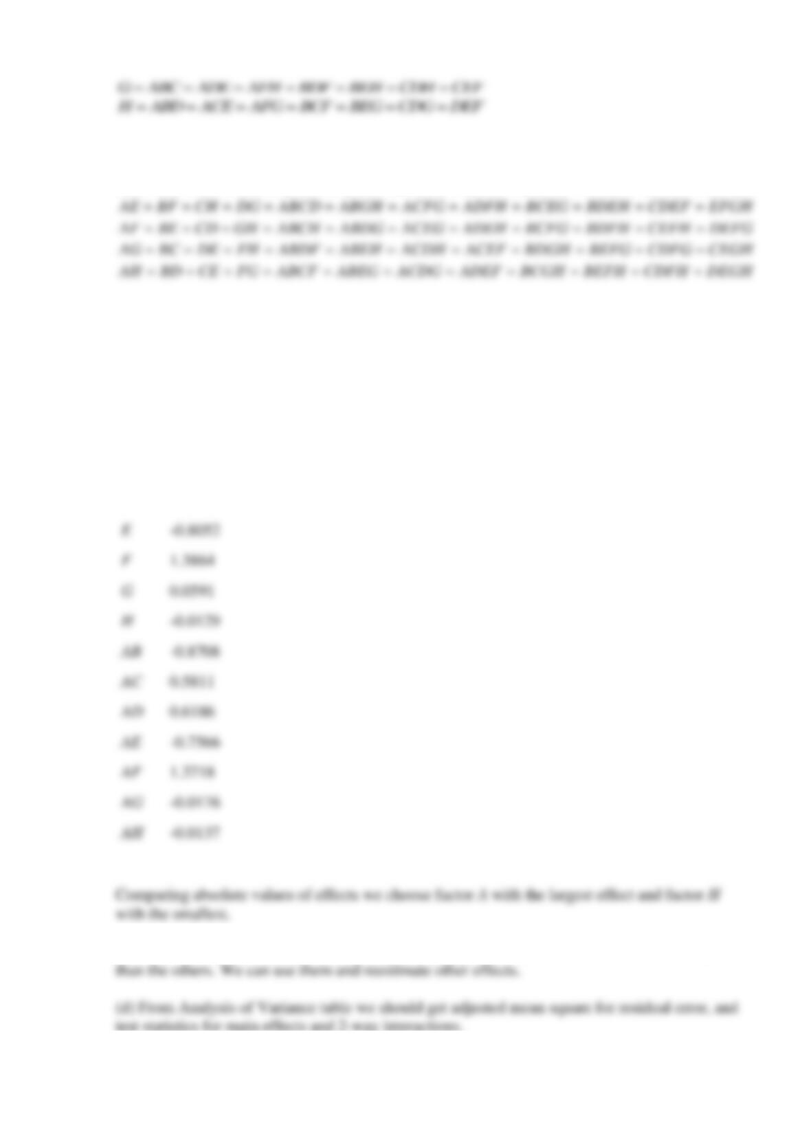
AB CG DH EF ACDE ACFH ADFG AEGH BCDF BCEH BDEG BFGH= = = = = = = = = = =
AC BG DF EH ABDE ABFH ADGH AEFG BCDH BCEF CDEG CFGH= = = = = = = = = = =
AD BH CF EG ABCE ABFG ACGH AEFH BCDG BDEF CDEH DFGH= = = = = = = = = = =
AG BC DE FH ABDF ABEH ACDH ACEF BDGH BEFG CDFG CEGH= = = = = = = = = = =
AH BD CE FG ABCF ABEG ACDG ADEF BCGH BEFH CDFH DEGH= = = = = = = = = = =
(b) From “Estimated Effects and Coefficients” outflow we can get values of effects:
A
1.4497
B
-0.8624
C
0.6034
D
0.6519
E
-0.8052
F
1.3864
G
0.0591
H
-0.0129
-0.8708
0.5811
0.6186
-0.7566
1.3718
-0.0176
-0.0137
(c) From the effects table and the normal probability plot effects G, H, AG, and AH are smaller

Important parts of table:
Source
DF
AdjMS
F
P
Main Effects
6
~4.14
995.39
0
Reserve Problems Chapter 14 Section 10 Problem 2
An experiment to optimize culture medium factors to enhance phenazine-1-carboxylic acid
(PCA) production was described. A
51
2−
fractional factorial design was conducted with factors
soybean meal, glucose, corn steep liquor, ethanol, and MgSO4. Rows below the horizontal line in
the table (coded with zeros) correspond to center points.
Run
1
X
2
X
3
X
4
X
5
X
Production (g/L)
1
−
−
−
−
+
1575.5
2
+
−
−
−
−
2201.4
3
−
+
−
−
−
1813.9
4
+
+
−
−
+
2164.1
5
−
−
+
−
−
1739.6
6
+
−
+
−
+
2483.2
7
−
+
+
−
+
2159.1
8
+
+
+
−
−
2257.7
9
−
−
−
+
−
1386.3
10
+
−
−
+
+
1967.8
11
−
+
−
+
+
1306
12
+
+
−
+
−
2486.9
13
−
−
+
+
+
2374.9
14
+
−
+
+
−
2932.7
15
−
+
+
+
−
2458.9
16
+
+
+
+
+
3204.9
17
0
0
0
0
0
2630.4
18
0
0
0
0
0
2571.6
19
0
0
0
0
0
2734.5
2-Way Interactions
5
~4.14
757.11
0
Residual Error
4
Total

20
0
0
0
0
0
2480.4
21
0
0
0
0
0
2662.5
Variable
Component
Levels (g/L)
−1
0
+1
1
X
Soybean meal
30
45
60
2
X
Ethanol
12
18
24
3
X
Corn steep liquor
7
10.5
14
4
X
Glucose
10
15
20
5
X
MgSO4
0
1
2
(a) What are the generator and resolution of this design?
(b) Analyze factor effects. Determine the effect and test statistic for each main factor.
(c) Choose significant effects to build a model to predict production in terms of the actual factor
levels.
(d) Build a model using only significant effects. What are the coefficients to predict production
in terms of the actual factor level?
SOLUTION
(b) Estimated effects and coefficients for production:
Term
Effect
Coef
SECoef
T
P
Constant
2157.06
23.97
89.99
0.000
A
611
305.28
23.97
12.74
0.000
B
149
74.38
23.97
3.10
0.036
C
589
294.32
23.97
12.28
0.000
D
215.49
107.74
23.97
4.50
0.011
E
23.97
0.918
23.97
0.197
BC
-11
-5.61
23.97
-0.23
0.827
BD
50
24.99
23.97
1.04
0.356
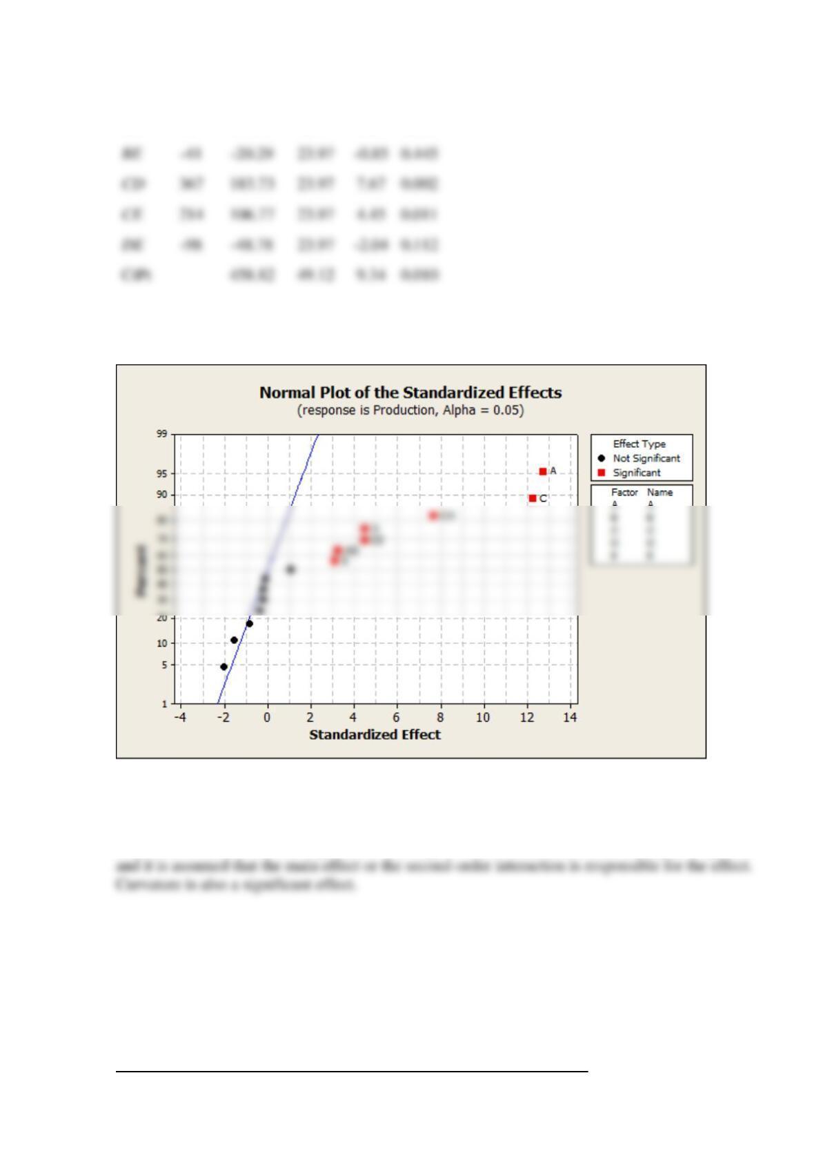
Normal plot of effects:
(c) According to the table of effects and normal plot, main effects A, B, C, D and two-factor
interactions AD, CD, CE are significant. The higher-order interaction in each alias pair is ignored
(d) Because CE is a significant interaction, to maintain a hierarchical model, factor E (MgSO4) is
also added to the model.
Estimated Effects and Coefficients for Production (coded units):
Term
Effect
Coef
SE Coef
T
P
BE
-41
23.97
-0.85
0.445
106.77
23.97
4.45
0.011
-98
23.97
-2.04
0.112
CtPt
458.82
49.12
9.34
0.010
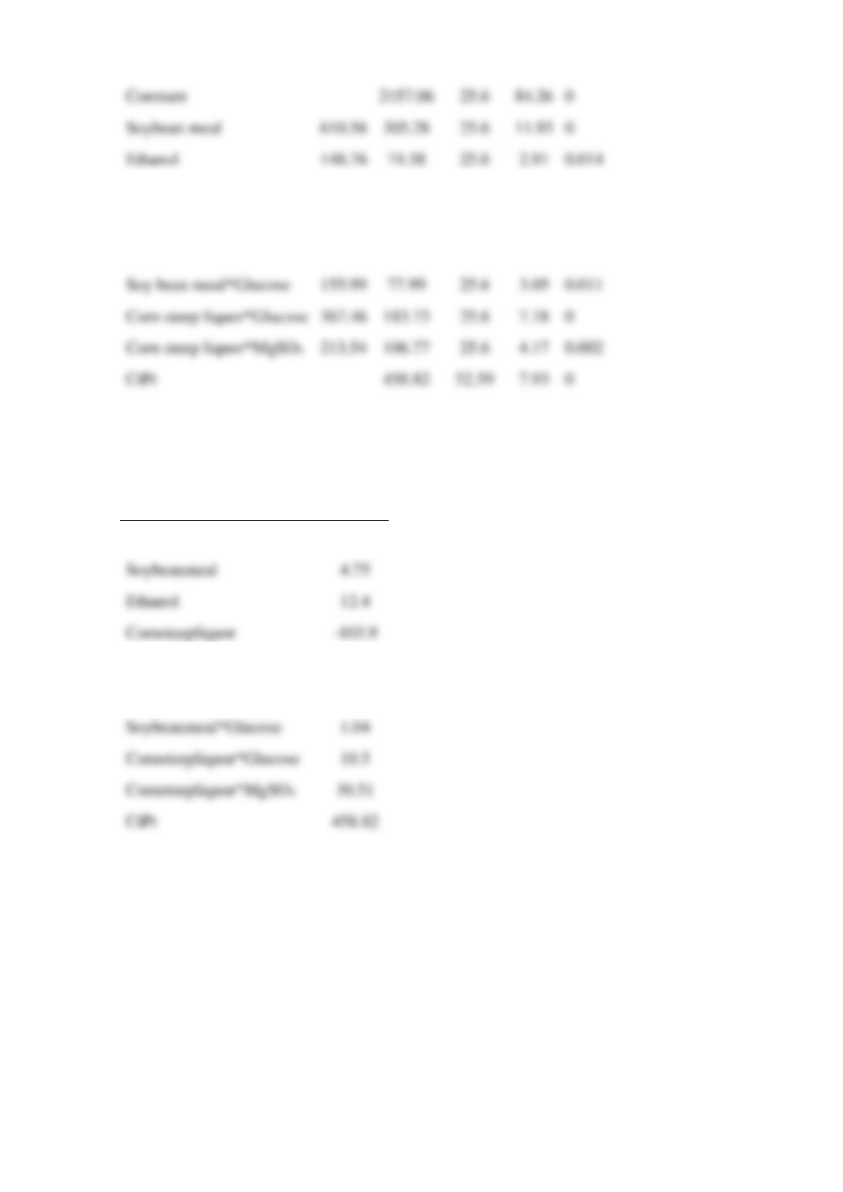
Corn steep liquor
588.64
294.32
25.6
11.5
0
Glucose
215.49
107.74
25.6
4.21
0.001
MgSO4
-5.24
-2.62
25.6
-0.1
0.92
Soy bean meal*Glucose
155.99
25.6
3.05
0.011
Corn steep liquor*Glucose
367.46
183.73
25.6
7.18
0
Corn steep liquor*MgSO4
213.54
106.77
25.6
4.17
0.002
CtPt
458.82
52.59
7.93
0
Estimated Coefficients for Production using data in uncoded units:
Term
Coef
Constant
2490.33
Soybeanmeal
4.75
Ethanol
12.4
Cornsteepliquor
-103.9
Glucose
-135.49
MgSO4
-322.93
Soybeanmeal*Glucose
1.04
Cornsteepliquor*Glucose
10.5
Cornsteepliquor*MgSO4
CtPt
458.82
Reserve Problems Chapter 14 Section 10 Problem 3
An experiment to optimize the removal of TNT 2,4,6-trinitrotoluene (TNT) is described. TNT is
a predominant contaminant at ammunition plants, testing facilities and military zones. TNT
removal (TR) is measured by the percentage of the initial concentration removed (mg/kg-soil).
A
73
2−
fractional factorial design was conducted. The data are in the following table. Rows
below the horizontal line in the table correspond to center points.
Constant
2157.06
25.6
84.26
0
Soybean meal
610.56
305.28
25.6
11.93
0
Ethanol
148.76
25.6
2.91
0.014

Glucose
(g/L)
NH4Cl
(g/L)
Tween80
(g/L)
Slurry
(g/ml)
Temp
(°C)
Yeast
(g/L)
Inoculum
(vol.%)
Run
A
B
C
D
E
F
G
TR
1
2
0.1
5
20
35
0.2
10
90.5
2
8
0.1
5
20
20
0.2
5
80.1
3
8
0.1
1
20
35
0
10
92.3
4
2
0.1
5
40
35
0
5
82.9
5
2
0.1
1
40
20
0.2
10
68.1
6
8
0.5
1
20
20
0.2
10
90.4
7
2
0.5
1
40
35
0
10
71.6
8
8
0.1
1
40
35
0.2
5
79.5
9
8
0.5
5
40
35
0.2
10
86.5
10
2
0.5
5
40
20
0.2
5
84.1
11
8
0.5
5
20
35
0
5
91.3
12
2
0.5
1
20
35
0.2
5
89.7
13
8
0.5
1
40
20
0
5
78.1
14
2
0.1
1
20
20
0
5
90.4
15
2
0.5
5
20
20
0
10
91
16
8
0.1
5
40
20
0
10
83.6
17
5
0.3
3
30
27.5
0.1
7.5
85.6
18
5
0.3
3
30
27.5
0.1
7.5
89.7
19
5
0.3
3
30
27.5
0.1
7.5
88.3
(a) What are the generators and the complete defining relation for this design?
(b) What is the resolution of this design?
(c) Analyze factor effects. Determine the value of F-statistic for the following sources.
(d) Develop a regression model to predict removal in terms of the actual factor levels.
(e) Use the model developed in part (d). Determine the coefficients to predict production in
terms of the actual factor level.
SOLUTION
(a), (b)
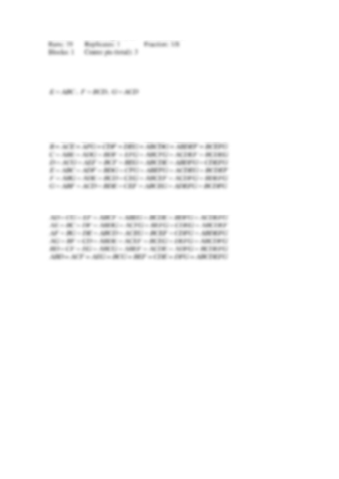
Factors: 7 Base Design: 7, 16 Resolution: IV
Design Generators:
Alias Structure:
I ABCE ABFG ACDG ADEF BCDF BDEG CEFG= = = = = = =
A BCE BFG CDG DEF ABCDF ABDEG ACEFG= = = = = = =
AB CE FG ACDF ADEG BCDG BDEF ABCEFG= = = = = = =
AC BE DG ABDF AEFG BCFG CDEF ABCDEG= = = = = = =
AD CG EF ABCF ABEG BCDE BDFG ACDEFG= = = = = = =
AF BG DE ABCD ACEG BCEF CDFG ABDEFG= = = = = = =
AG BF CD ABDE ACEF BCEG DEFG ABCDFG= = = = = = =
ABD ACF AEG BCG BEF CDE DFG ABCDEFG= = = = = = =
(c)
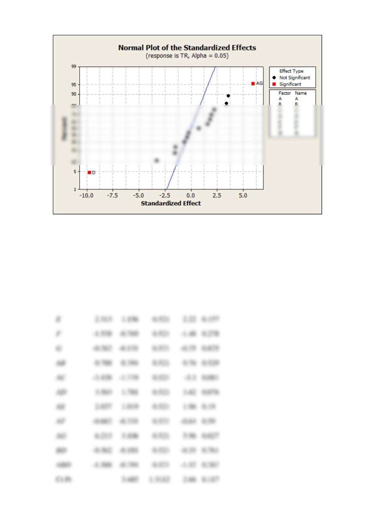
Estimated Effects and Coefficients for TR (coded units):
Term
Effect
Coef
SE Coef
T
P
Constant
84.381
0.521
161.96
0
A
1.687
0.844
0.521
1.62
0.247
B
1.912
0.956
0.521
1.84
0.208
C
3.737
1.869
0.521
3.59
0.07
D
-10.163
-5.081
0.521
-9.75
0.01
E
2.313
1.156
0.521
2.22
0.157
F
-1.538
-0.769
0.521
-1.48
0.278
G
-0.262
-0.131
0.521
-0.25
0.825
0.788
0.394
0.521
0.76
0.529
-3.438
-1.719
0.521
0.081
3.563
1.781
0.521
3.42
0.076
2.037
1.019
0.521
1.96
0.19
-0.662
-0.331
0.521
-0.64
0.59
6.213
3.106
0.521
5.96
0.027
-0.362
-0.181
0.521
-0.35
0.761
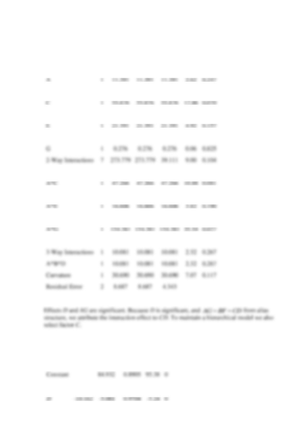
Analysis of Variance for TR (coded units)
Source
DF
Seq SS
Adj SS
Adj MS
F
P
Main Effects
7
526.124
526.124
75.161
17.30
0.056
B
1
14.631
14.631
14.631
3.37
0.208
C
1
55.876
55.876
55.876
12.86
0.070
D
1
413.106
413.106
413.106
95.11
0.010
E
1
21.391
21.391
21.391
4.92
0.157
F
1
9.456
9.456
9.456
2.18
0.278
G
1
0.276
0.276
0.276
0.06
0.825
2-Way Interactions
7
273.779
273.779
39.111
9.00
0.104
A*B
1
2.481
2.481
2.481
0.57
0.529
A*C
1
47.266
47.266
47.266
10.88
0.081
A*D
1
50.766
50.766
50.766
11.69
0.076
A*E
1
16.606
16.606
16.606
3.82
0.190
A*F
1
1.756
1.756
1.756
0.40
0.590
A*G
1
154.381
154.381
154.381
35.54
0.027
B*D
1
0.526
0.526
0.526
0.12
0.761
3-Way Interactions
1
10.081
10.081
10.081
2.32
0.267
A*B*D
1
10.081
10.081
10.081
2.32
0.267
Curvature
1
30.690
30.690
30.690
7.07
0.117
Residual Error
2
8.687
8.687
4.343
(d), (e) Estimated Effects and Coefficients for TR (coded units)
Term
Effect
Coef
SE Coef
T
P
Constant
84.932
95.38
0
C
3.737
1.869
0.9704
1.93
0.073
D
-10.162
0.9704
0
A
1
11.391
11.391
11.391
2.62
0.247
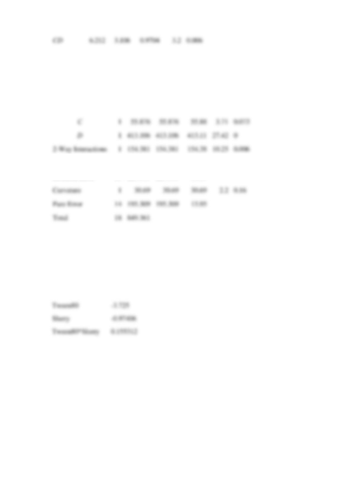
Analysis of Variance for TR (coded units)
Source
DF
Seq SS
Adj SS
Adj MS
F
P
Main Effects
2
468.981
468.981
234.49
15.56
0
1
55.88
0.073
1
413.106
413.106
413.11
27.42
0
2-Way Interactions
1
154.381
154.381
154.38
10.25
0.006
CD
1
154.381
154.381
154.38
10.25
0.006
Residual Error
15
225.999
225.999
15.07
Curvature
1
30.69
0.16
Pure Error
14
195.309
195.309
13.95
Total
18
849.361
To predict removal in terms of the actual factor levels we should use estimated coefficients in
uncoded units:
Term
Coef
Constant
111.35
Tween80
-3.725
Slurry
-0.97406
Tween80*Slurry
0.155312
Reserve Problems Chapter 14 Section 11 Problem 1
Consider the first-order model
1 2 3 4
12 1.25 2.00 1.6 0.85y x x x x= + − + −
, where
11
i
x−
.
(a) Find the direction of steepest ascent (as a vector).
(b) Assume that the current design is centered at the point (0, 0, 0, 0). Determine the point that is
three units from the current center point in the direction of steepest ascent.
SOLUTION
6.212
0.006
(b) The point along the path of steepest descent that is 3 units away from (0, 0, 0, 0) is given by:
Reserve Problems Chapter 14 Section 11 Problem 2
Consider two responses
1
y
and
2
y
which are functions of two inputs
1
x
and
2
x
.
22
1 2 1 1 2
2.1 4.1 3.8y x x x x= − − +
22
2 1 2
( 2.0) ( 2.7)y x x= − + −
How feasible is it to minimize both
1
y
and
2
y
with values for
1
x
and
2
x
?
Determine the minimum point.
If it is possible to minimize both
1
y
and
2
y
, but with different values for
1
x
and
2
x
, determine
the minimum point for
1
y
; if it is impossible to minimize both
1
y
and
2
y
, enter “none”.
SOLUTION
It is impossible to minimize
1
y
, and
2
y
is minimized at
Reserve Problems Chapter 14 Section 11 Problem 3
Two responses
1
y
and
2
y
are related to two inputs
1
x
and
2
x
by the models
( ) ( )
22
1 1 2
5 2 3y x x= + − + −
and
2 2 1 3y x x= − +
.
Suppose that the objectives are
114y
and
26y
.
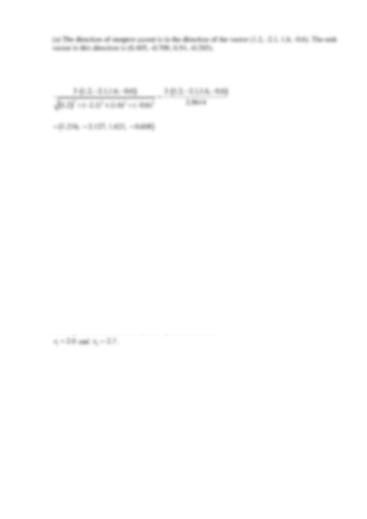
(a) Choose the right feasible set of operating conditions for
1
x
and
2
x
:
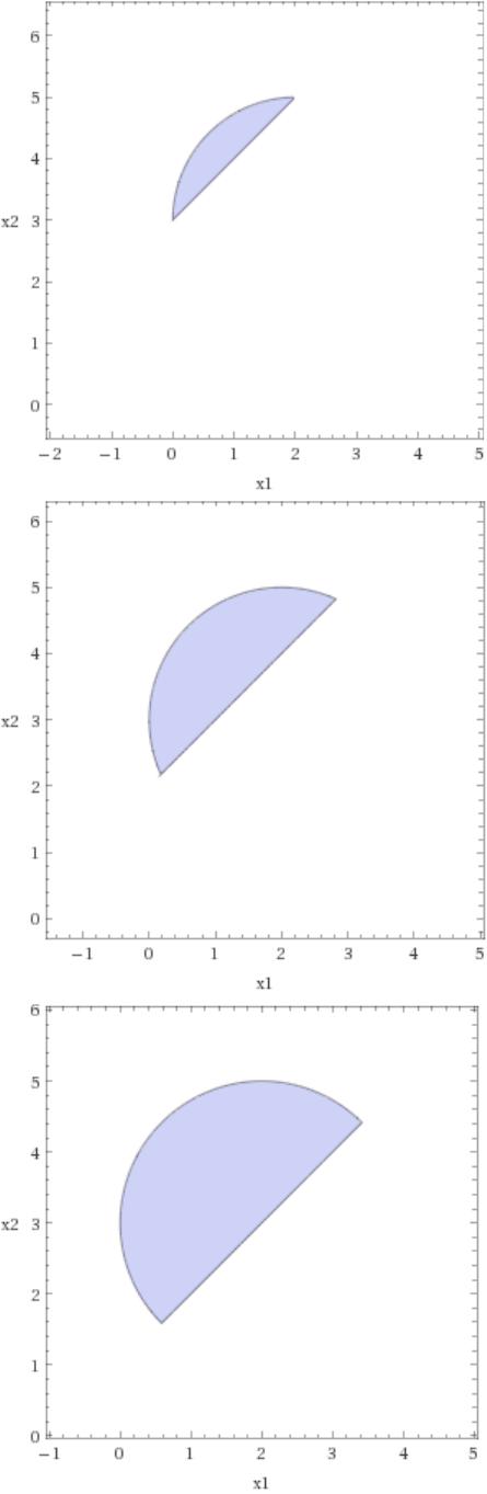
A
B
C
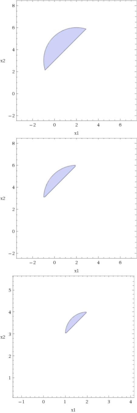
D
E
F

(b) Determine the point
( )
12
, xx
that yields
26y
and minimizes
1
y
.
SOLUTION
(a) The region
114y
is a circle in
( )
12
, xx
space centered at the point (2, 3) with radius 3. The
(b) Minimum of
1
y
is the point of feasible region from (a), closest to the point (2, 3) and located
Reserve Problems Chapter 14 Section 11 Problem 4
We used response surface methodology to generate surface roughness prediction models for
turning EN 24T steel (290 BHN). The data and factors are shown in the following tables.
Coding
Trial
Speed
(m/min)
Feed
(mm/rev)
Depth of cut
(mm)
1
x
2
x
3
x
Surface roughness
(μm)
1
36
0.15
0.5
-1
-1
-1
1.8
2
117
0.15
0.5
1
-1
-1
1.233
3
36
0.4
0.5
-1
1
-1
5.3
4
117
0.4
0.5
1
1
-1
5.067
5
36
0.15
1.125
-1
-1
1
2.133
6
117
0.15
1.125
1
-1
1
1.45
7
36
0.4
1.125
-1
1
1
6.233
8
117
0.4
1.125
1
1
1
5.167
9
65
0.25
0.75
0
0
0
2.433
10
65
0.25
0.75
0
0
0
2.3
11
65
0.25
0.75
0
0
0
2.367
12
65
0.25
0.75
0
0
0
2.467
13
28
0.25
0.75
2−
0
0
3.633
14
150
0.25
0.75
2
0
0
2.767