
13–21
Applied Statistics and Probability for Engineers,7th edition 2017
13–22
Cross-linker
level ———+———+———+———+
0.5 (—*—)
1 (—*—)
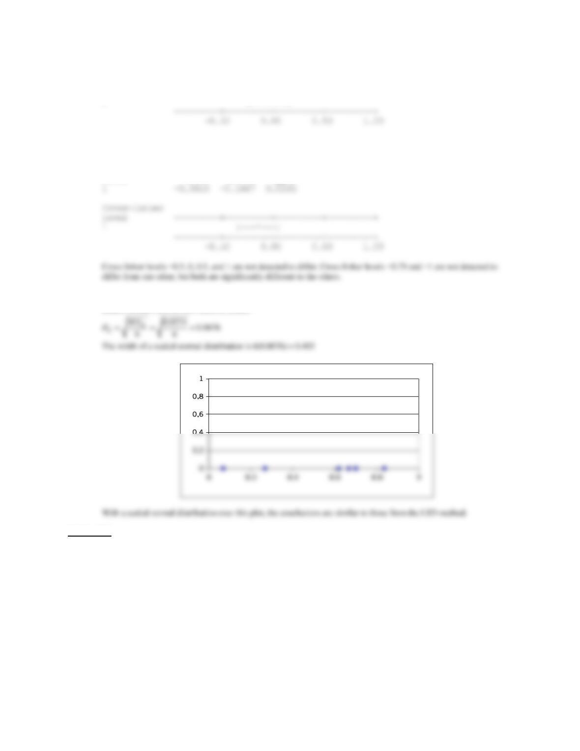
Cross-linker level = 0.5 subtracted from:
Cross-linker
level Lower Center Upper
(b) The mean values are
8.0667, 8.2667, 8.6167, 8.7, 8.8333, 8.6667
Section 13.3
13.3.1 An article in the Journal of the Electrochemical Society [1992, Vol. 139(2), pp. 524–532)] describes an experiment
to investigate the low-pressure vapor deposition of polysilicon. The experiment was carried out in a large-capacity
reactor at Sematech in Austin, Texas. The reactor has several wafer positions, and four of these positions were selected
at random. The response variable is film thickness uniformity. Three replicates of the experiment were run, and the data
are as follows:
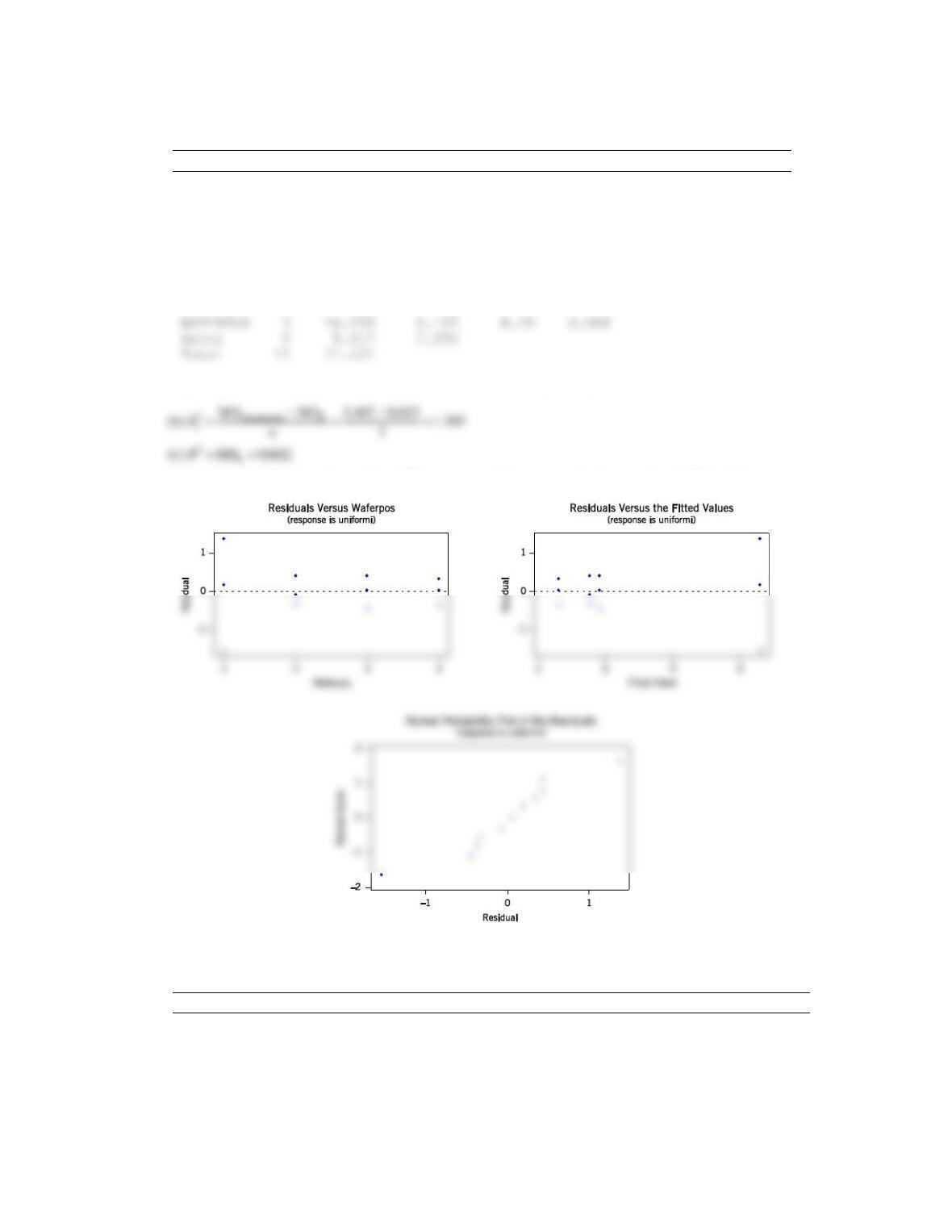
(a) Is there a difference in the wafer positions? Use
= 0.05.
(b) Estimate the variability due to wafer positions.
(c) Estimate the random error component.
Applied Statistics and Probability for Engineers,7th edition 2017
13–23
(d) Analyze the residuals from this experiment and comment on model adequacy.
Wafer Position
Uniformity
1
2.76
5.67
4.49
2
1.43
1.70
2.19
3
2.34
1.97
1.47
4
0.94
1.36
1.65
(a)
Analysis of Variance for UNIFORMITY
Source DF SS MS F P
Reject H0, and conclude that there are significant differences among wafer positions.
(d) Greater variability at wafer position 1. There is some slight curvature in the normal probability plot.
13.3.2 A textile mill has a large number of looms. Each loom is supposed to provide the same output of cloth per minute. To
investigate this assumption, five looms are chosen at random, and their output is measured at different times. The
following data are obtained:
Loom
Output (lb/min)
1
4.0
4.1
4.2
4.0
4.1
2
3.9
3.8
3.9
4.0
4.0
3
4.1
4.2
4.1
4.0
3.9
4
3.6
3.8
4.0
3.9
3.7
5
3.8
3.6
3.9
3.8
4.0
Applied Statistics and Probability for Engineers,7th edition 2017
13–24
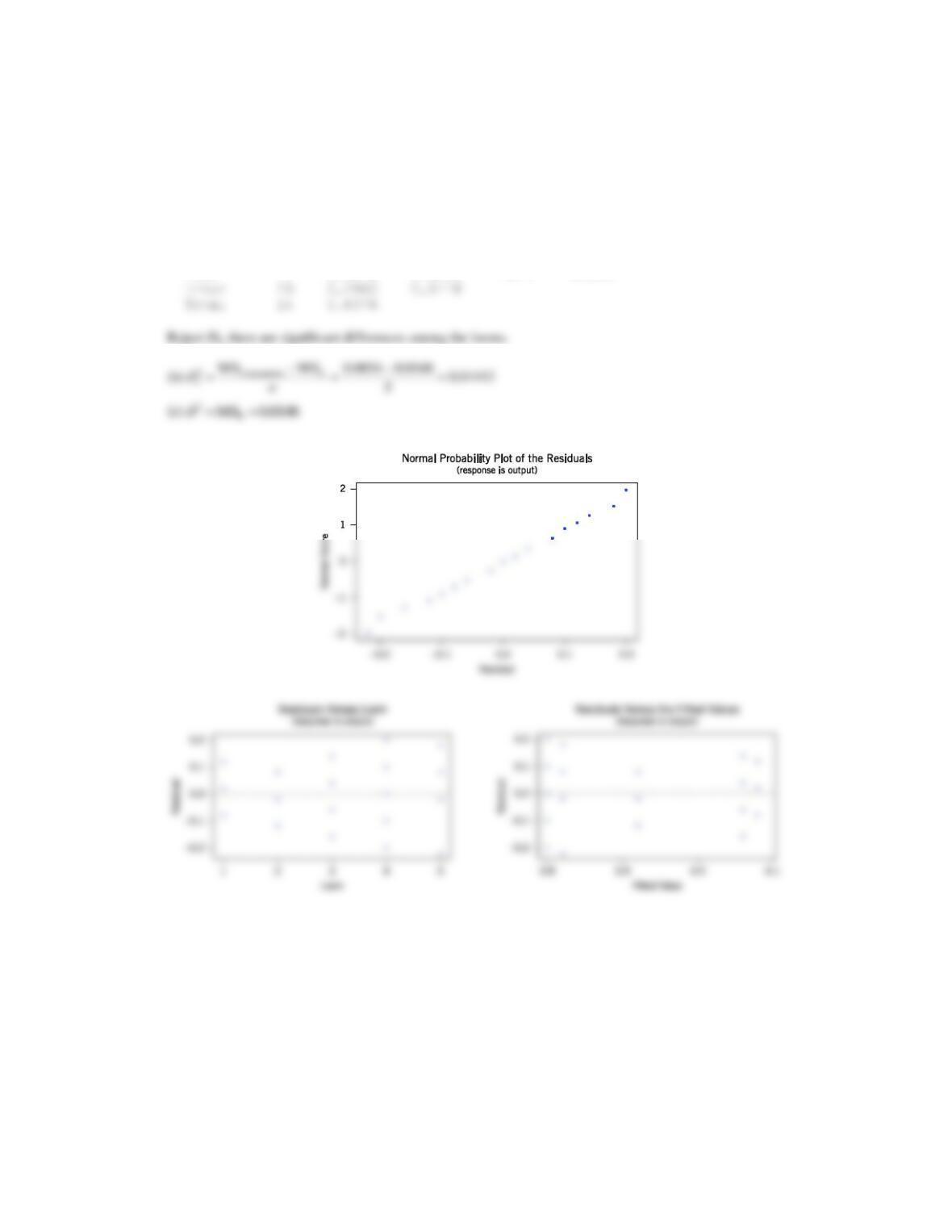
(a) Are the looms similar in output? Use
= 0.05.
(b) Estimate the variability between looms.
(c) Estimate the experimental error variance.
(d) Analyze the residuals from this experiment and check for model adequacy.
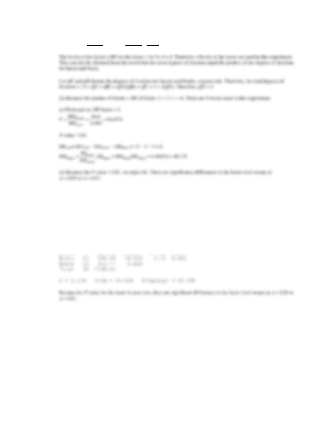
(a) Analysis of Variance for OUTPUT
Source DF SS MS F P
LOOM 4 0.3416 0.0854 5.77 0.003
(d) Residuals are acceptable.
Applied Statistics and Probability for Engineers,7th edition 2017
13.3.3 In the book Bayesian Inference in Statistical Analysis (1973, John Wiley and Sons) by Box and Tiao, the total product
yield for five samples was determined randomly selected from each of six randomly chosen batches of raw material.
Batch
Yield (in grams)
1
1545
1440
1440
1520
1580
2
1540
1555
1490
1560
1495
3
1595
1550
1605
1510
1560
4
1445
1440
1595
1465
1545
5
1595
1630
1515
1635
1625
6
1520
1455
1450
1480
1445
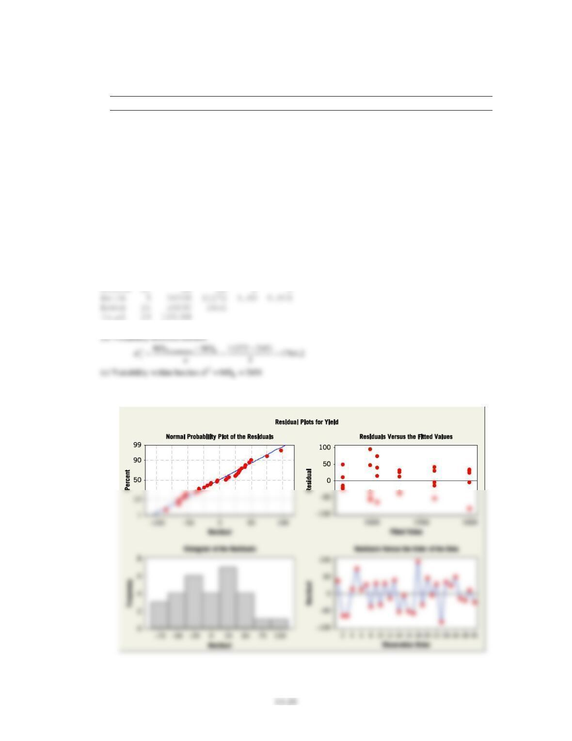
(a) Do the different batches of raw material significantly affect mean yield? Use
= 0.01.
(b) Estimate the variability between batches.
(c) Estimate the variability between samples within batches.
(d) Analyze the residuals from this experiment and check for model adequacy.
(a) Yes, the different batches of raw material significantly affect mean yield at
= 0.01 because the P–value is small.
(d) The normal probability plot and the residual plots show that the model assumptions are reasonable.
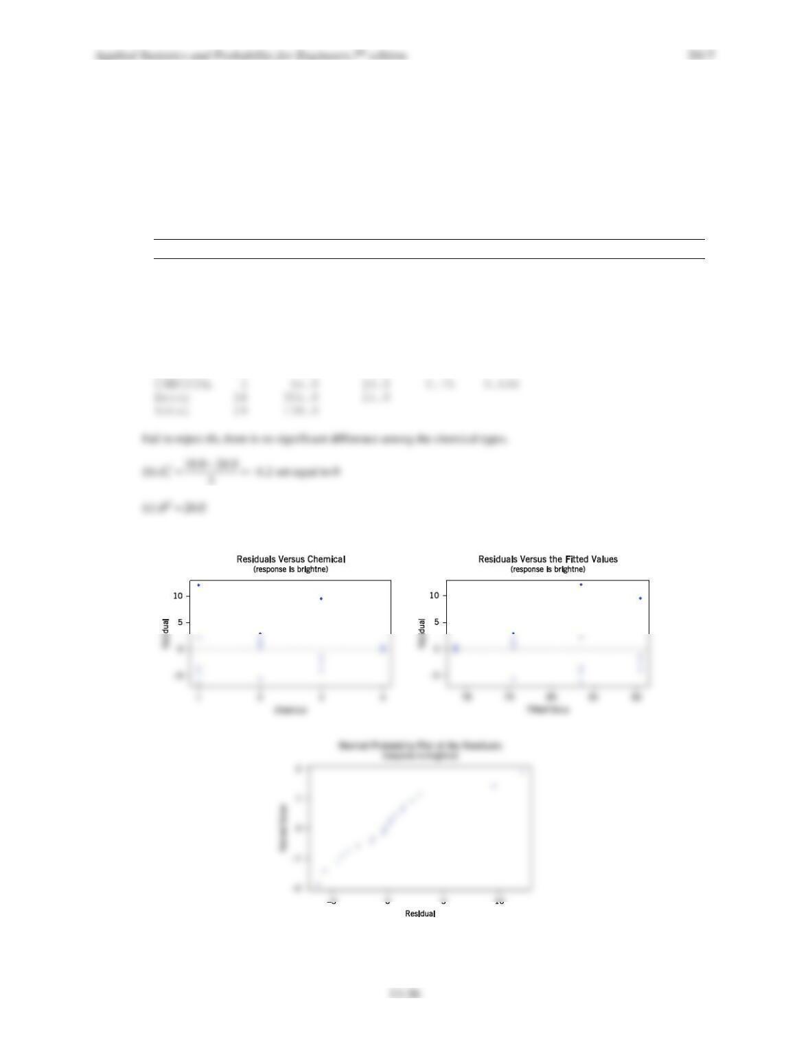
13.3.4 An article in the Journal of Quality Technology [1981, Vol. 13(2), pp. 111–114)] described an experiment that
investigated the effects of four bleaching chemicals on pulp brightness. These four chemicals were selected at random
from a large population of potential bleaching agents. The data are as follows:
(a) Is there a difference in the chemical types? Use
= 0.05.
(b) Estimate the variability due to chemical types.
(c) Estimate the variability due to random error.
(d) Analyze the residuals from this experiment and comment on model adequacy.
Chemical
Pulp Brightness
1
77.199
74.466
92.746
76.208
82.876
2
80.522
79.306
81.914
80.346
73.385
3
79.417
78.017
91.596
80.802
80.626
4
78.001
78.358
77.544
77.364
77.386
(a) Analysis of Variance for BRIGHTNENESS
Source DF SS MS F P
(d) Variability is smaller in chemical 4. There is some curvature in the normal probability plot.
13–27
13.3.5 Consider the vapor-deposition experiment described in Exercise 13-34.
(a) Estimate the total variability in the uniformity response.
(b) How much of the total variability in the uniformity response is due to the difference between positions in the
reactor?
(c) To what level could the variability in the uniformity response be reduced if the position-to-position variability in
the Reactor could be eliminated? Do you believe this is a substantial reduction?
13.3.6 Consider the cloth experiment described in Exercise 13-35.
(a) Estimate the total variability in the output response.
(b) How much of the total variability in the output response is due to the difference between looms?
(c) To what level could the variability in the output response be reduced if the loom-to-loom variability could be
eliminated? Do you believe this is a significant reduction?
From 13-35 we have
−−
= = =
==
2Treatments E
2
E
MS MS 0.0854 0.0148
ˆ0.01412
5
ˆMS 0.0148
n
Section 13.4
13.4.1 Consider the following computer output from a RCBD.
Source
DF
SS
MS
F
P
Factor
?
193.800
64.600
?
?
Block
3
464.218
154.739
Error
?
?
4.464
Total
15
698.190
(a) How many levels of the factor were used in this experiment?
(b) How many blocks were used in this experiment?
(c) Fill in the missing information. Use bounds for the P-value.
(d) What conclusions would you draw if
= 0.05? What would you conclude if
= 0.01?
Applied Statistics and Probability for Engineers,7th edition 2017
13–28
(a)
===
factor facto
factor factor
r
factor factor
SS SS 193.8
,3
DF MS 64
M D = .6
SF
13.4.2 Exercise 13.2.4 introduced you to an experiment to investigate the potential effect of consuming chocolate on
cardiovascular health. The experiment was conducted as a completely randomized design, and the exercise asked you
to use the ANOVA to analyze the data and draw conclusions. Now, assume that the experiment had been conducted as
an RCBD with the subjects considered as blocks. Analyze the data using this assumption. What conclusions would you
draw (using
= 0.05) about the effect of the different types of chocolate on cardiovascular health? Would your
conclusions change if
= 0.01?
The output from computer software follows.
Source DF SS MS F P
Factor 2 1952.64 976.322 147.35 0.000
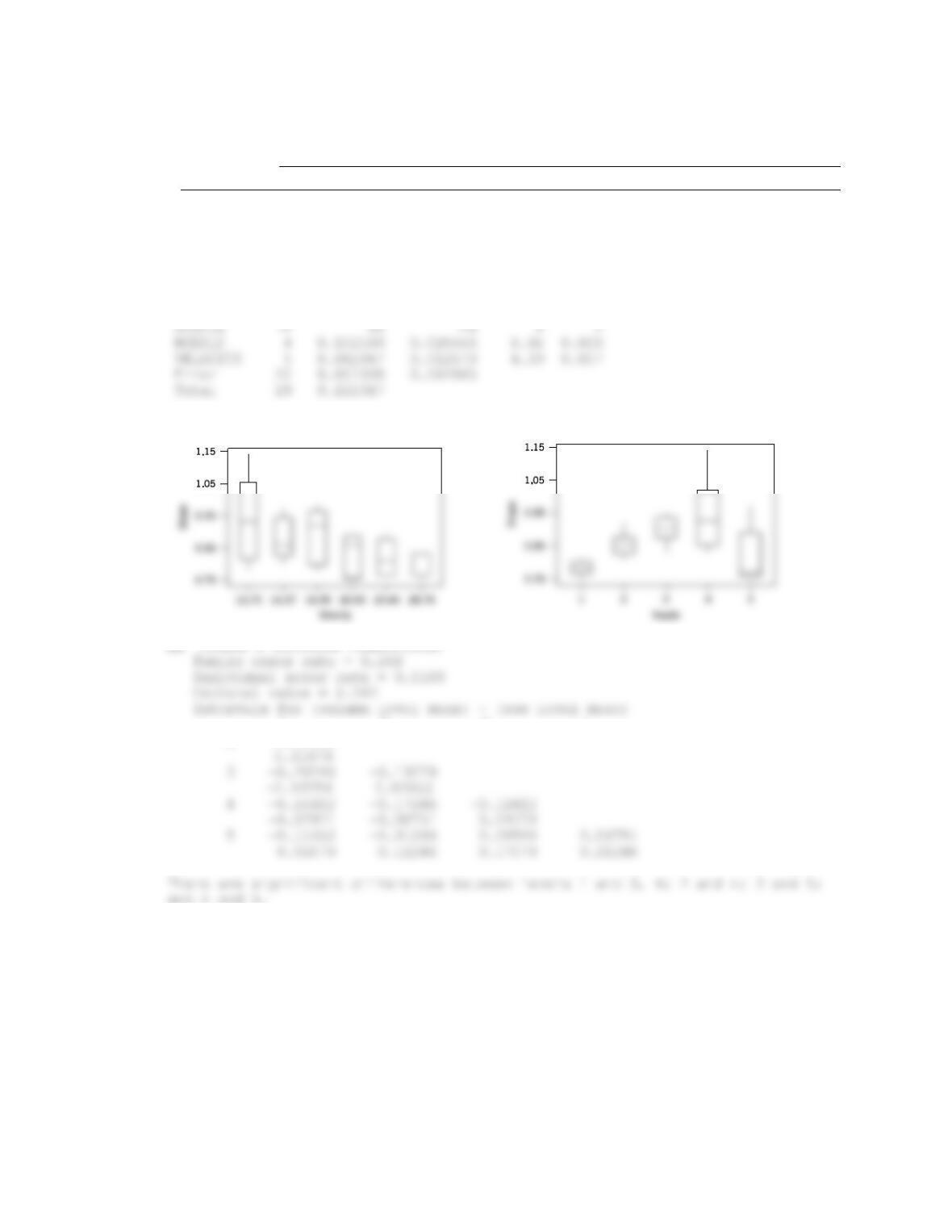
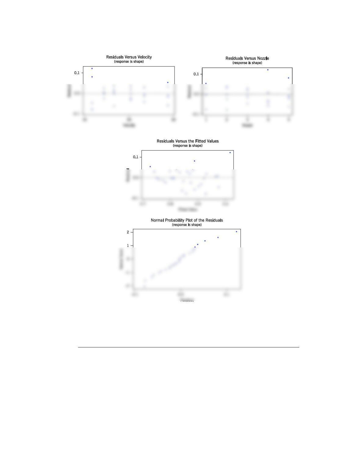
13.4.3 In “The Effect of Nozzle Design on the Stability and Performance of Turbulent Water Jets” (Fire Safety Journal,
August 1981, Vol. 4), C. Theobald described an experiment in which a shape measurement was determined for several
different nozzle types at different levels of jet efflux velocity. Interest in this experiment focuses primarily on nozzle
type, and velocity is a nuisance factor. The data are as follows:
(a) Does nozzle type affect shape measurement? Compare the nozzles with box plots and the analysis of variance.
(b) Use Fisher’s LSD method to determine specific differences among the nozzles. Does a graph of the average
(or standard deviation) of the shape measurements versus nozzle type assist with the conclusions?
Applied Statistics and Probability for Engineers,7th edition 2017
13–29
(c) Analyze the residuals from this experiment.
Jet Efflux Velocity (m/s)
Nozzle Type
11.73
14.37
16.59
20.43
23.46
28.74
1
0.78
0.80
0.81
0.75
0.77
0.78
2
0.85
0.85
0.92
0.86
0.81
0.83
3
0.93
0.92
0.95
0.89
0.89
0.83
4
1.14
0.97
0.98
0.88
0.86
0.83
5
0.97
0.86
0.78
0.76
0.76
0.75
(a) Analysis of Variance for SHAPE
Reject H0, nozzle type affects shape measurement.
(b) Fisher’s pairwise comparisons
1 2 3 4
2 -0.15412
Applied Statistics and Probability for Engineers,7th edition 2017
13–30
(c) The residual analysis shows that there is some inequality of variance. The normal probability plot is acceptable.
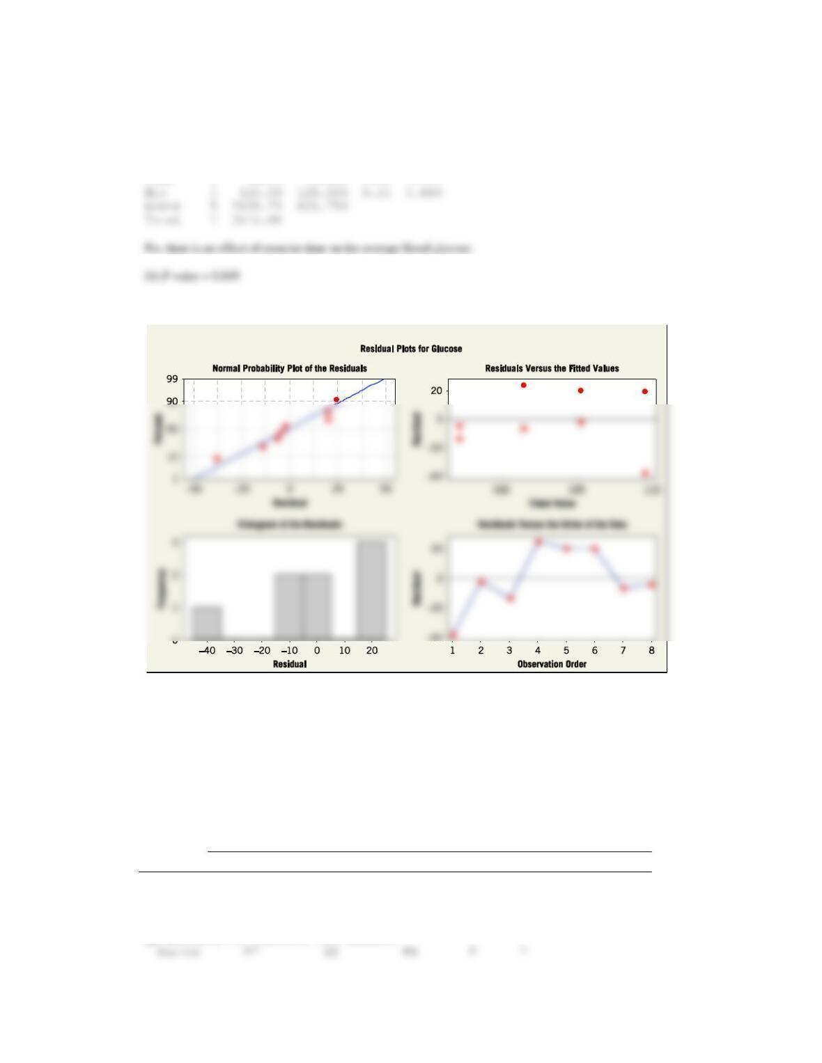
13.4.4 An article in Quality Engineering [“Designed Experiment to Stabilize Blood Glucose Levels” (1999–2000,
Vol. 12, pp. 83–87)] described an experiment to minimize variations in blood glucose levels. The treatment was the
exercise time on a Nordic Track cross-country skier (10 or 20 min). The experiment was blocked for time
of day. The data were as follows:
Exercise (min)
Time of Day
Average Blood Glucose
10
pm
71.5
10
am
103.0
20
am
83.5
20
pm
126.0
10
am
125.5
10
pm
129.5
20
pm
95.0
20
am
93.0
(a) Is there an effect of exercise time on the average blood glucose? Use
= 0.05.
Applied Statistics and Probability for Engineers,7th edition 2017
13–31
(b) Find the P-value for the test in part (a).
(c) Analyze the residuals from this experiment.
(a) Analysis of variance for Glucose
Source DF SS MS F P
Time 1 36.13 36.125 0.06 0.819
(c) The normal probability plot and the residual plots show that the model assumptions are reasonable.
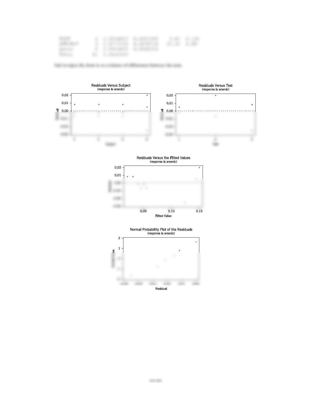
13.4.5 An article in the American Industrial Hygiene Association Journal (1976, Vol. 37, pp. 418–422) described a field test
for detecting the presence of arsenic in urine samples. The test has been proposed for use among forestry workers
because of the increasing use of organic arsenics in that industry. The experiment compared the test as performed by
both a trainee and an experienced trainer to an analysis at a remote laboratory. Four subjects were selected for testing
and are considered as blocks. The response variable is arsenic content (in ppm) in the subject’s urine. The data are as
follows:
(a) Is there any difference in the arsenic test procedure?
(b) Analyze the residuals from this experiment.
Subject
Test
1
2
3
4
Trainee
0.05
0.05
0.04
0.15
Trainer
0.05
0.05
0.04
0.17
Lab
0.04
0.04
0.03
0.10
(a) Analysis of Variance for ARSENIC
Applied Statistics and Probability for Engineers,7th edition 2017
(b) Some indication of variability increasing with the magnitude of the response.
13–33
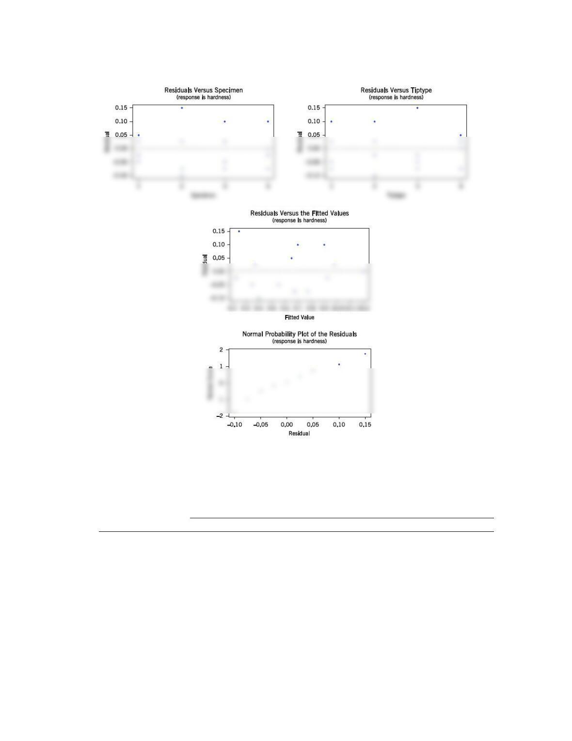
13.4.6 In Design and Analysis of Experiments, 8th edition (John Wiley & Sons, 2012), D. C. Montgomery described an
experiment that determined the effect of four different types of tips in a hardness tester on the observed hardness of a
metal alloy. Four specimens of the alloy were obtained, and each tip was tested once on each specimen, producing the
following data:
Specimen
Type of Tip
1
2
3
4
1
9.3
9.4
9.6
10.0
2
9.4
9.3
9.8
9.9
3
9.2
9.4
9.5
9.7
4
9.7
9.6
10.0
10.2
(a) Is there any difference in hardness measurements between the tips?
(b) Use Fisher’s LSD method to investigate specific differences between the tips.
(c) Analyze the residuals from this experiment.
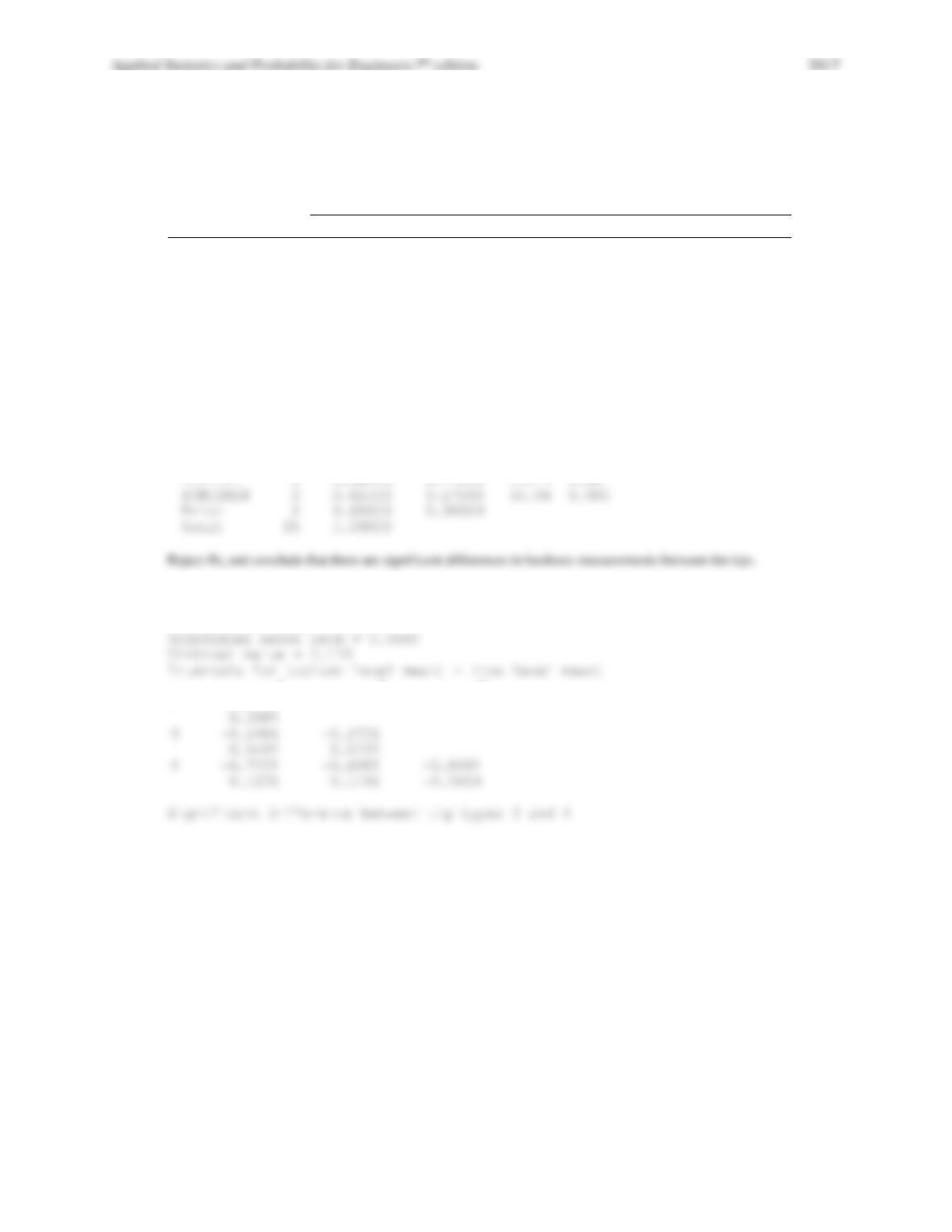
(a) Analysis of Variance of HARDNESS
Source DF SS MS F P
(b)
Fisher’s pairwise comparisons
Family error rate = 0.184
1 2 3
2 -0.4481
Applied Statistics and Probability for Engineers,7th edition 2017
13–34
(c) Residuals are acceptable.
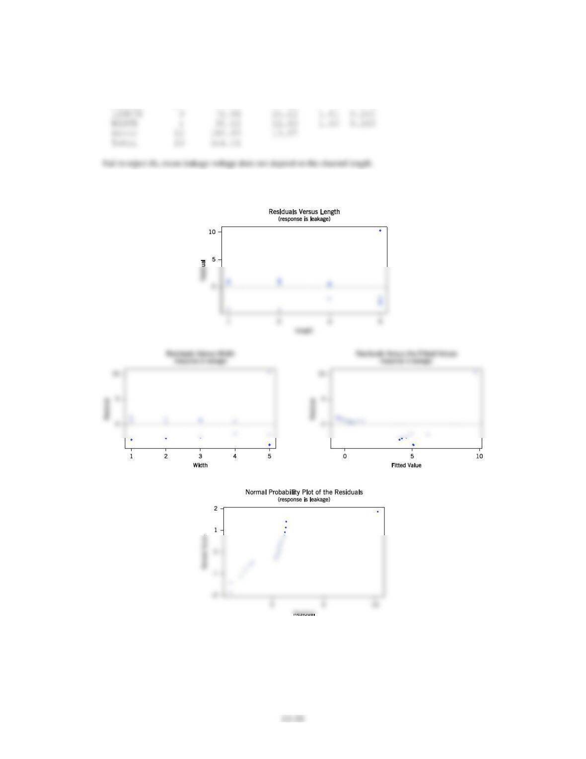
13.4.7 An experiment was conducted to investigate leaking current in a SOS MOSFETS device. The purpose of the
experiment was to investigate how leakage current varies as the channel length changes. Four channel lengths were
selected. For each channel length, five different widths were also used, and width is to be considered a nuisance factor.
The data are as follows:
Channel
Length
Width
1
2
3
4
5
1
0.7
0.8
0.8
0.9
1.0
2
0.8
0.8
0.9
0.9
1.0
3
0.9
1.0
1.7
2.0
4.0
4
1.0
1.5
2.0
3.0
20.0
(a) Test the hypothesis that mean leakage voltage does not depend on the channel length using
= 0.05.
(b) Analyze the residuals from this experiment. Comment on the residual plots.
(c) The observed leakage voltage for channel length 4 and width 5 was erroneously recorded. The correct observation is
4.0. Analyze the corrected data from this experiment. Is there evidence to conclude that mean leakage voltage increases
with channel length?
Applied Statistics and Probability for Engineers,7th edition 2017
A version of the electronic data file has the reading for length 4 and width 5 as 2. It should be 20.
(a) Analysis of Variance for LEAKAGE
Source DF SS MS F P
(b) One unusual observation in width 5, length 4. There are some problems with the normal probability plot, including
the unusual observation.