
Applied Statistics and Probability for Engineers,7th edition 2017
13-1
CHAPTER 13
Section 13.2
13.2.1 Consider the following computer output.
Source
DF
SS
MS
F
P-value
Factor
?
117.4
39.1
?
?
Error
16
396.8
?
Total
19
514.2
(a) How many levels of the factor were used in this experiment?
(b) How many replicates did the experimenter use?
(c) Fill in the missing information in the ANOVA table. Use bounds for the P-value.
(d) What conclusions can you draw about differences in the factor-level means?
13.2.2 Consider the following computer output for an experiment. The factor was tested over four levels.
Source
DF
SS
MS
F
P-value
Factor
?
?
330.4716
4.42
?
Error
?
?
?
Total
31
?
(a) How many replicates did the experimenter use?
(b) Fill in the missing information in the ANOVA table. Use bounds for the P-value.
(c) What conclusions can you draw about differences in the factor-level means?
13-2
13.2.3 In Design and Analysis of Experiments, 8th edition (John Wiley & Sons, 2012), D. C. Montgomery described an
experiment in which the tensile strength of a synthetic fiber was of interest to the manufacturer. It is suspected that
strength is related to the percentage of cotton in the fiber. Five levels of cotton percentage were used, and five
replicates were run in random order, resulting in the following data.
Observations
Cotton
Percentage
1
2
3
4
5
15
7
7
15
11
9
20
12
17
12
18
18
25
14
18
18
19
19
30
19
25
22
19
23
35
7
10
11
15
11
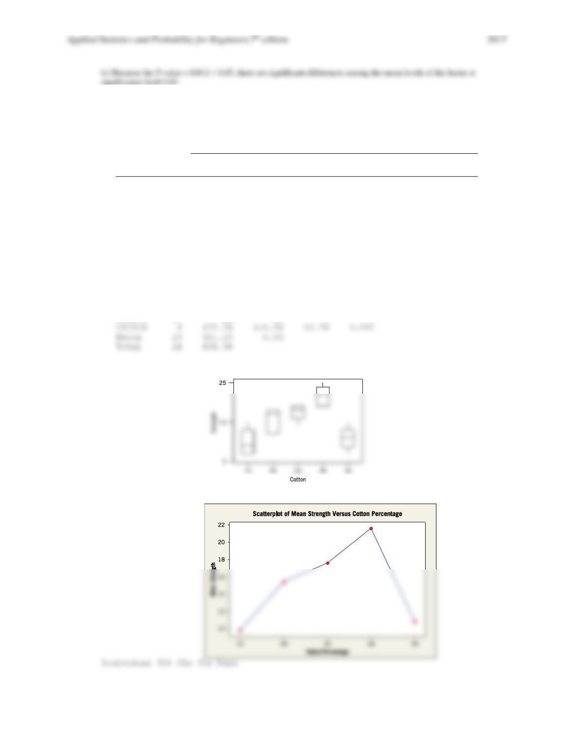
(a) Does cotton percentage affect breaking strength? Draw comparative box plots and perform an analysis of variance.
Use
= 0.05.
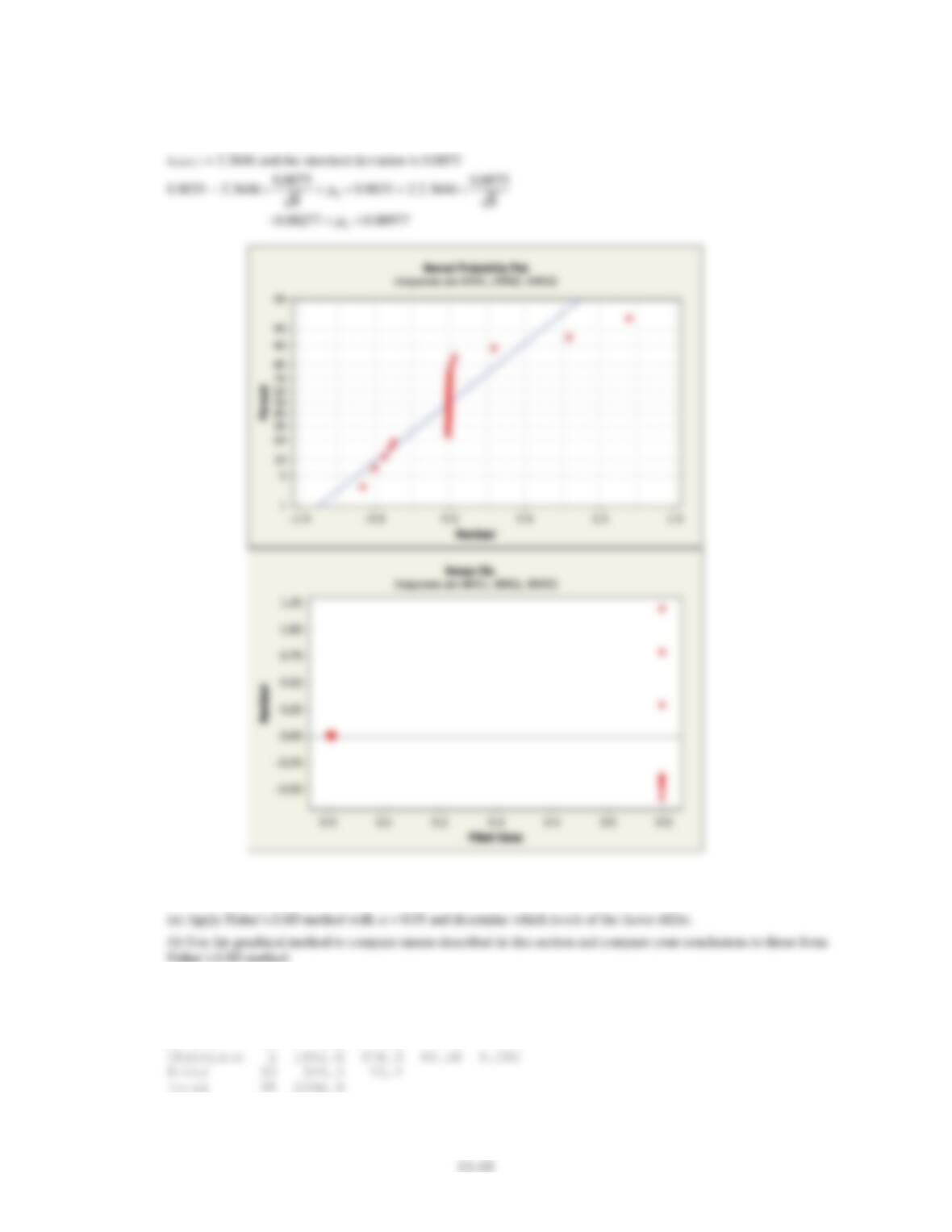
(b) Plot average tensile strength against cotton percentage and interpret the results.
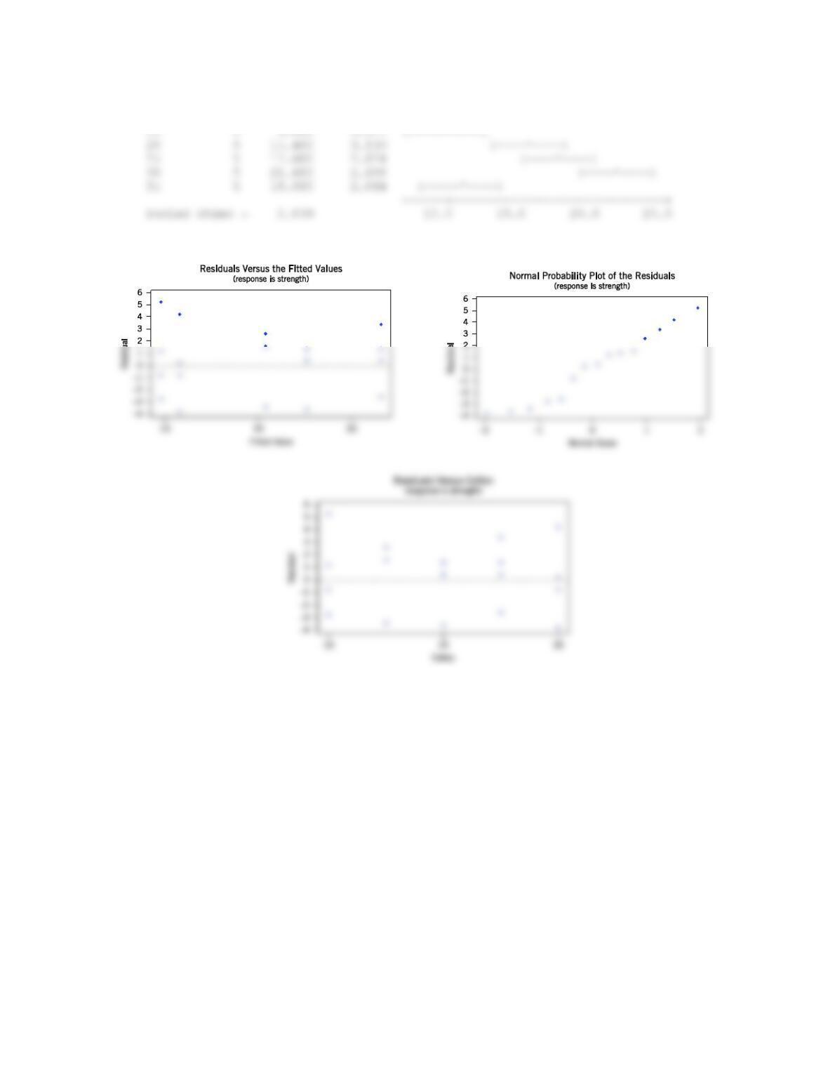
(c) Analyze the residuals and comment on model adequacy.
(a) Analysis of Variance for STRENGTH
Source DF SS MS F P
Reject H0 and conclude that cotton percentage affects mean breaking strength.
(b) Tensile strength seems to increase up to 30% cotton and declines at 35% cotton.
Applied Statistics and Probability for Engineers,7th edition 2017
13-3
Based on Pooled StDev
Level N Mean StDev ——+———+———+———+
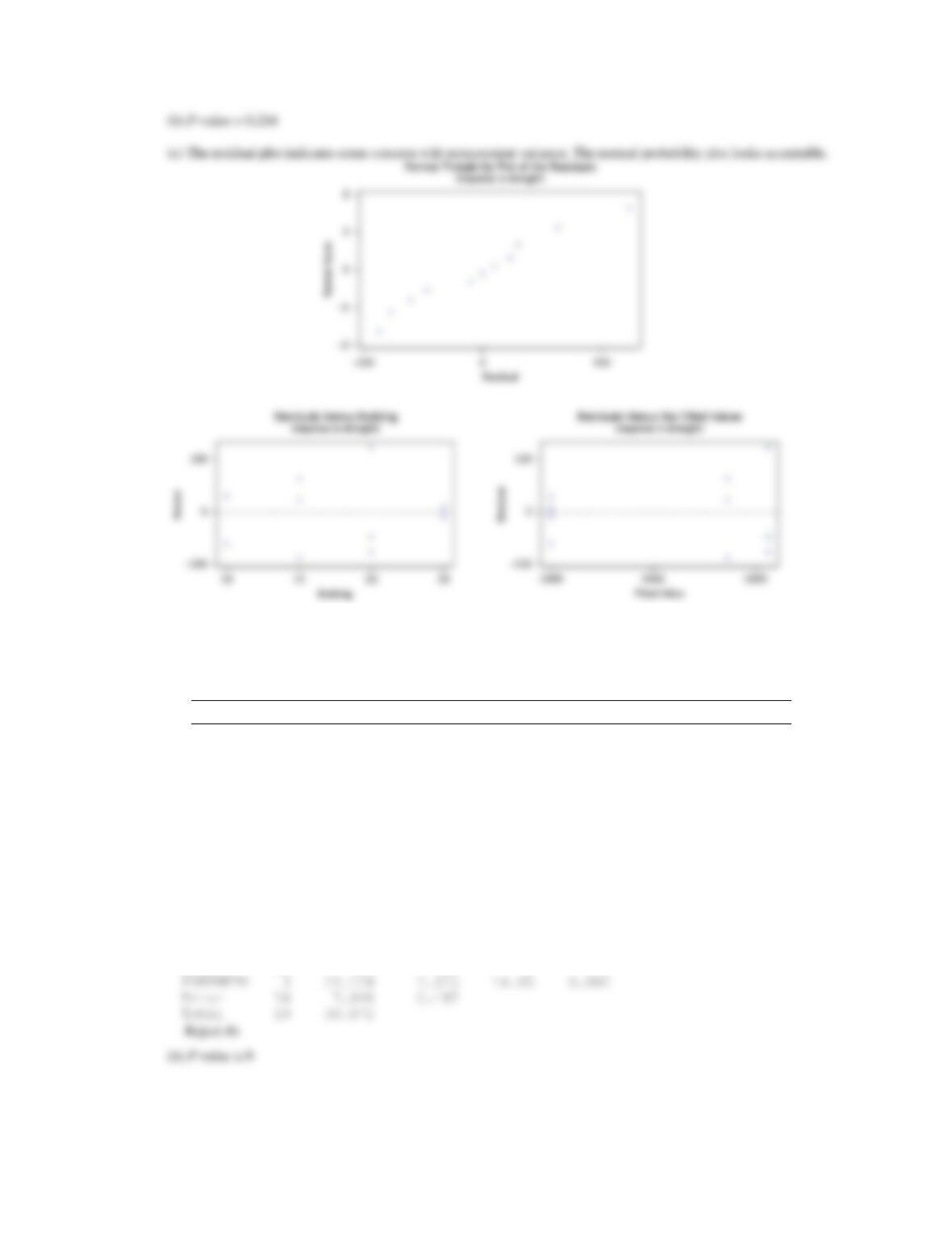
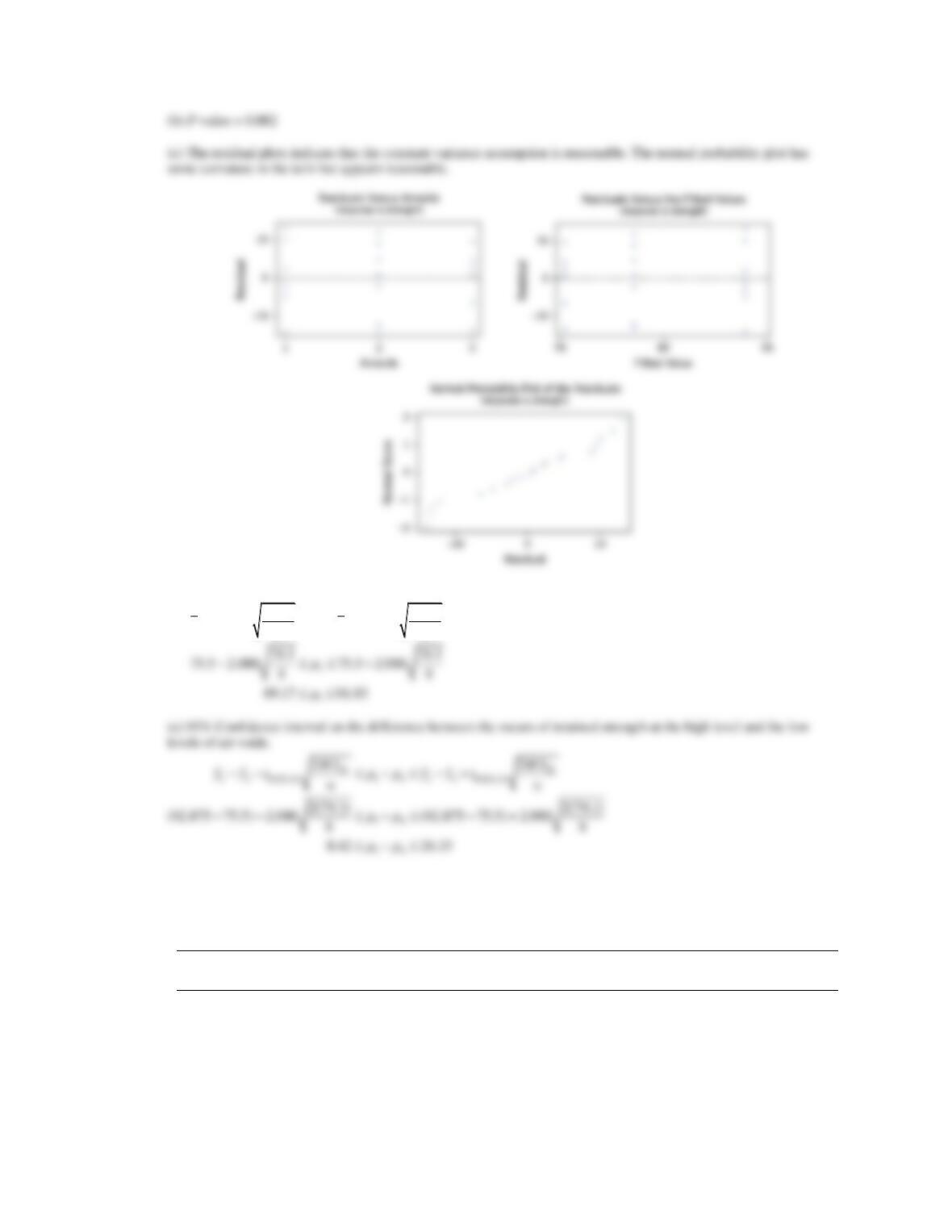
(c) The normal probability plot and the residual plots show that the model assumptions are reasonable.
13.2.4 An article in Nature describes an experiment to investigate the effect on consuming chocolate on cardiovascular health
(“Plasma Antioxidants from Chocolate,” 2003, Vol. 424, pp. 1013). The experiment consisted of using three different
types of chocolates: 100 g of dark chocolate, 100 g of dark chocolate with 200 ml of full-fat milk, and 200 g of milk
chocolate. Twelve subjects were used, seven women and five men with an average age range of 32.2 ± 1 years, an
average weight of 65.8 ± 3.1 kg, and body-mass index of 21.9 ± 0.4 kg m−2. On different days, a subject consumed one
of the chocolate-factor levels, and 1 hour later total antioxidant capacity of that person’s blood plasma was measured in
an assay. Data similar to those summarized in the article follow.
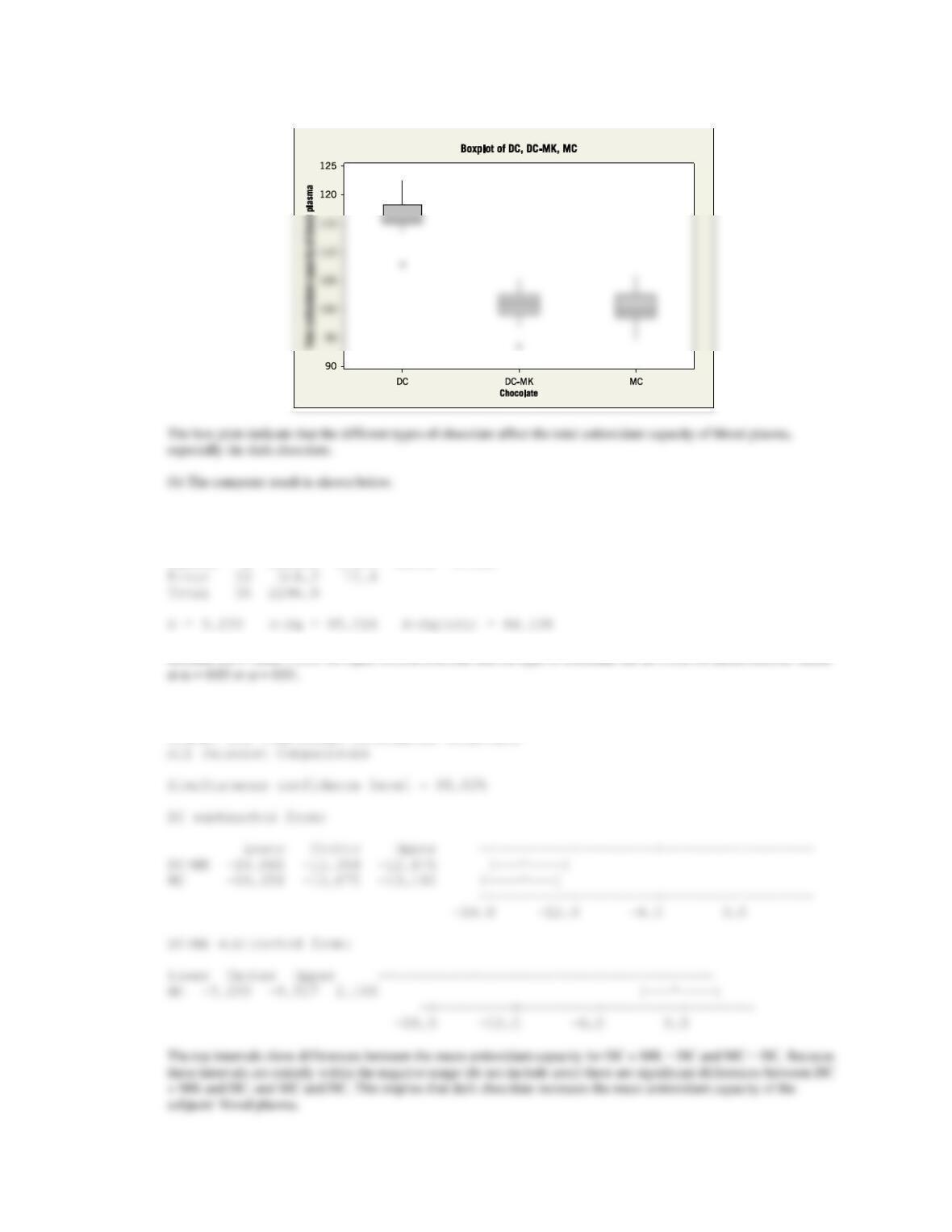
(a) Construct comparative box plots and study the data. What visual impression do you have from examining these
plots?
(b) Analyze the experimental data using an ANOVA. If
= 0.05, what conclusions would you draw? What would you
Conclude if
= 0.01?
(c) Is there evidence that the dark chocolate increases the mean antioxidant capacity of the subjects’ blood plasma?
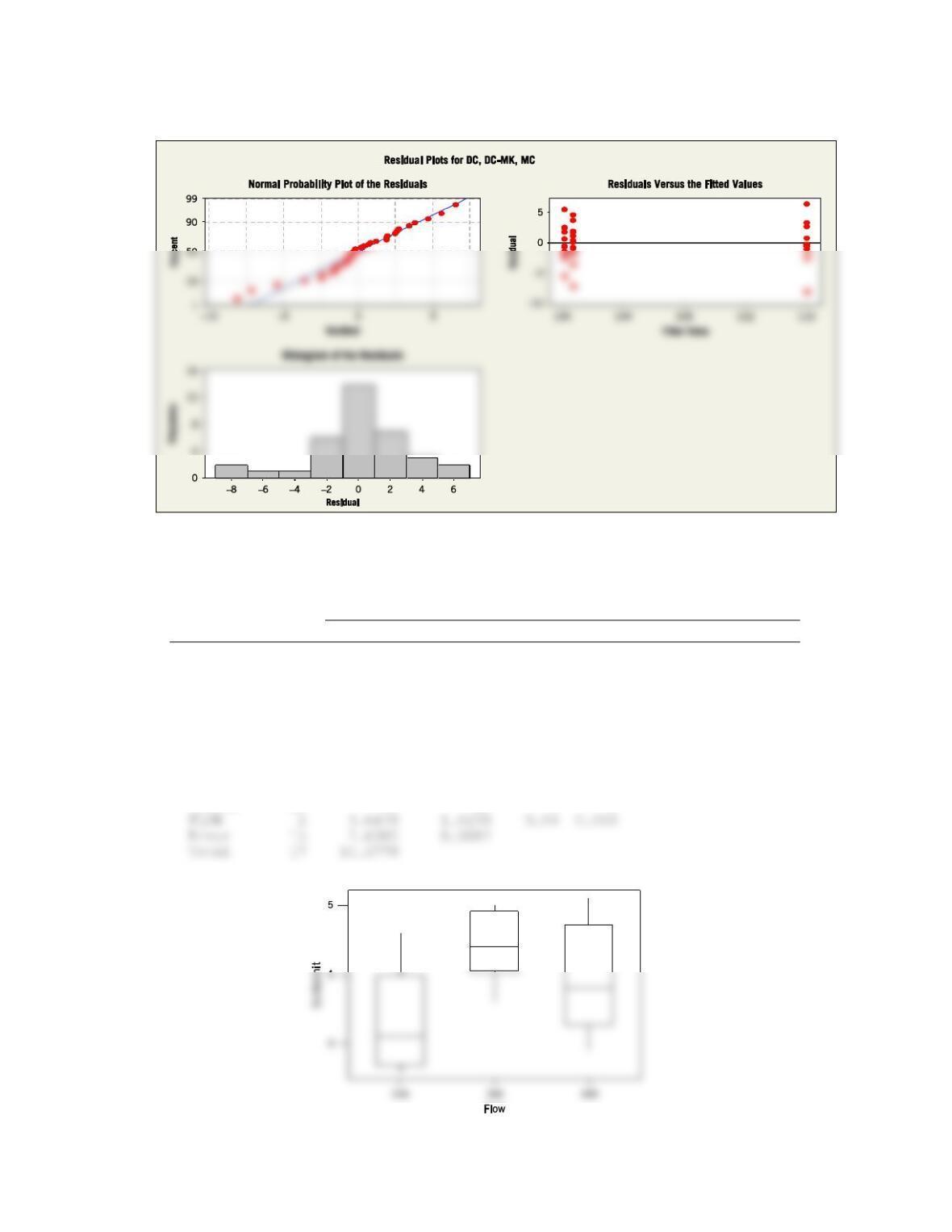
(d) Analyze the residuals from this experiment.
Applied Statistics and Probability for Engineers,7th edition 2017
13-4
a)
One-way ANOVA: DC, DC-MK, MC
Source DF SS MS F P
Factor 2 1952.6 976.3 93.58 0.000
Because the P-value < 0.01 we reject H0 and conclude that the type of chocolate has an effect on cardiovascular health
(c) The computer result is shown below.
Fisher 95% Individual Confidence Intervals
Applied Statistics and Probability for Engineers,7th edition 2017
13-5
(d) The normal probability plot and the residual plots show that the model assumptions are reasonable.
13.2.5 In “Orthogonal Design for Process Optimization and Its Application to Plasma Etching” (Solid State Technology, May
1987), G. Z. Yin and D. W. Jillie described an experiment to determine the effect of C2F6 flow rate on the uniformity of
the etch on a silicon wafer used in integrated circuit manufacturing. Three flow rates are used in the experiment, and
the resulting uniformity (in percent) for six replicates follows.
C2F6 Flow (SCCM)
Observations
1
2
3
4
5
6
125
2.7
4.6
2.6
3.0
3.2
3.8
160
4.9
4.6
5.0
4.2
3.6
4.2
200
4.6
3.4
2.9
3.5
4.1
5.1
(a) Does C2F6 flow rate affect etch uniformity? Construct box plots to compare the factor levels and perform the
analysis of variance. Use
= 0.05.
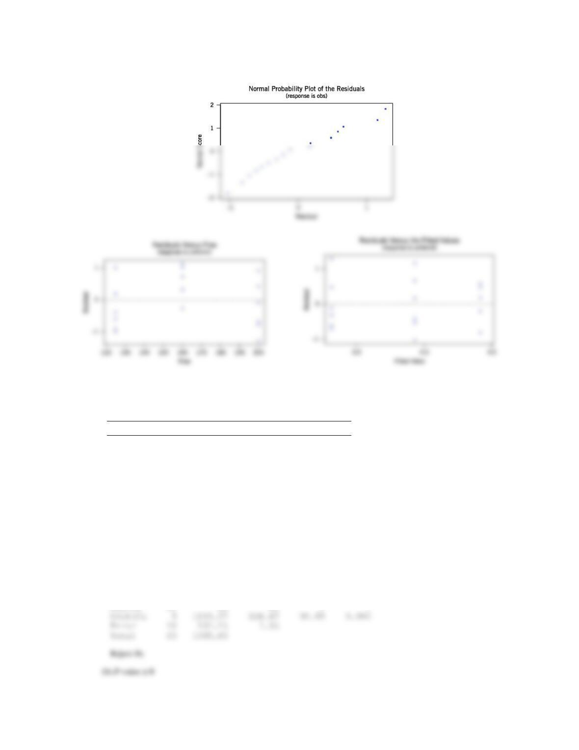
(b) Do the residuals indicate any problems with the underlying assumptions?
(a) Analysis of Variance for FLOW
Source DF SS MS F P
Fail to reject H0. There is no evidence that flow rate affects etch uniformity.
Applied Statistics and Probability for Engineers,7th edition 2017
13-6
(b) Residuals are acceptable.
13.2.6 An article in Environment International [1992, Vol. 18(4)] described an experiment in which the amount of radon
released in showers was investigated. Radon-enriched water was used in the experiment, and six different orifice
diameters were tested in shower heads. The data from the experiment are shown in the following table.
Orifice Diameter
Radon Released (%)
0.37
80
83
83
85
0.51
75
75
79
79
0.71
74
73
76
77
1.02
67
72
74
74
1.40
62
62
67
69
1.99
60
61
64
66
(a) Does the size of the orifice affect the mean percentage of radon released? Use α = 0.05.
(b) Find the P-value for the F-statistic in part (a).
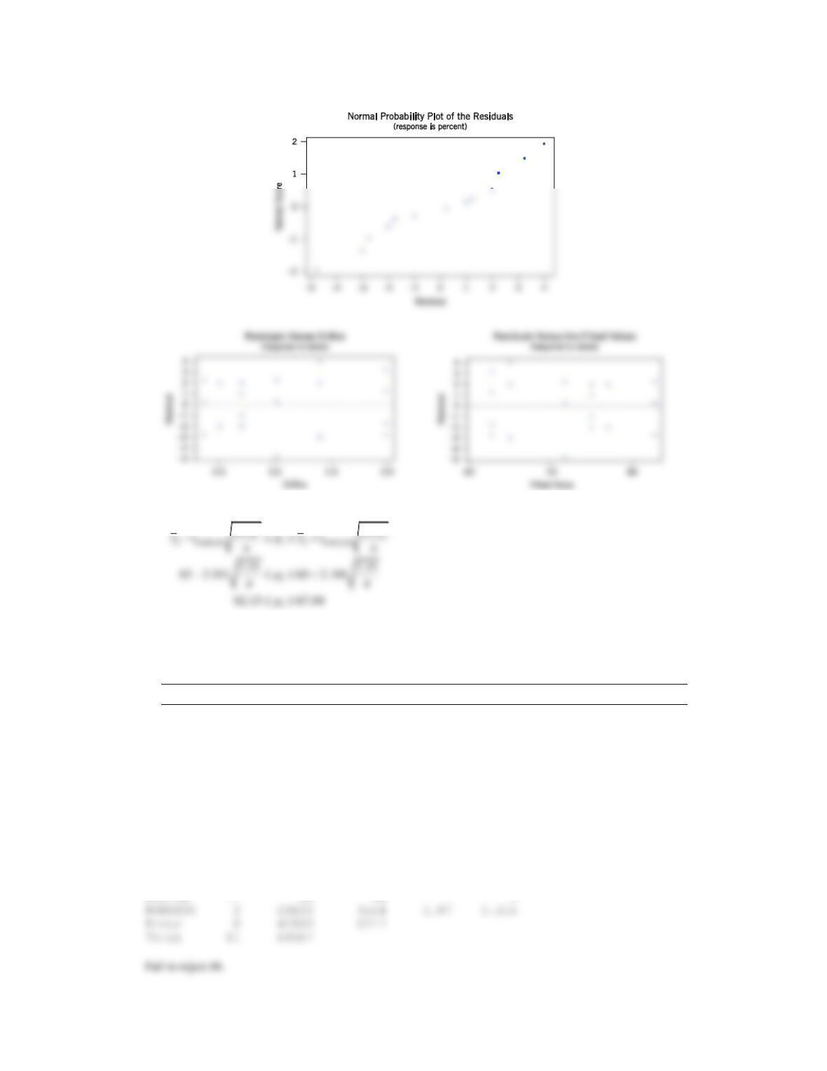
(c) Analyze the residuals from this experiment.
(d) Find a 95% confidence interval on the mean percent of radon released when the orifice diameter is 1.40.
(a) Analysis of Variance for ORIFICE
Source DF SS MS F P
Applied Statistics and Probability for Engineers,7th edition 2017
13-7
(c)
(d) 95% CI on the mean radon released when diameter is 1.40
M S M S
13.2.7 An article in the ACI Materials Journal (1987, Vol. 84, pp. 213–216) described several experiments investigating the
rodding of concrete to remove entrapped air. A 3-inch × 6-inch cylinder was used, and the number of times this rod was
used is the design variable. The resulting compressive strength of the concrete specimen is the response. The data are
shown in the following table.
Rodding Level
Compressive Strength
10
1530
1530
1440
15
1610
1650
1500
20
1560
1730
1530
25
1500
1490
1510
(a) Is there any difference in compressive strength due to the rodding level?
(b) Find the P-value for the F-statistic in part (a).
(c) Analyze the residuals from this experiment. What conclusions can you draw about the underlying model
assumptions?
(a) Analysis of Variance for STRENGTH
Source DF SS MS F P
Applied Statistics and Probability for Engineers,7th edition 2017
13-8
13.2.8 An article in the Materials Research Bulletin [1991, Vol. 26(11)] investigated four different methods of preparing the
superconducting compound PbMo6S8. The authors contend that the presence of oxygen during the preparation process
affects the material’s superconducting transition temperature Tc. Preparation methods 1 and 2 use techniques that are
designed to eliminate the presence of oxygen, and methods 3 and 4 allow oxygen to be present. Five observations on Tc
(in °K) were made for each method, and the results are as follows:
Preparation Method
Transition Temperature Tc (°K)
1
14.8
14.8
14.7
14.8
14.9
2
14.6
15.0
14.9
14.8
14.7
3
12.7
11.6
12.4
12.7
12.1
4
14.2
14.4
14.4
12.2
11.7
(a) Is there evidence to support the claim that the presence of oxygen during preparation affects the mean transition
temperature? Use
= 0.05.
(b) What is the P-value for the F-test in part (a)?
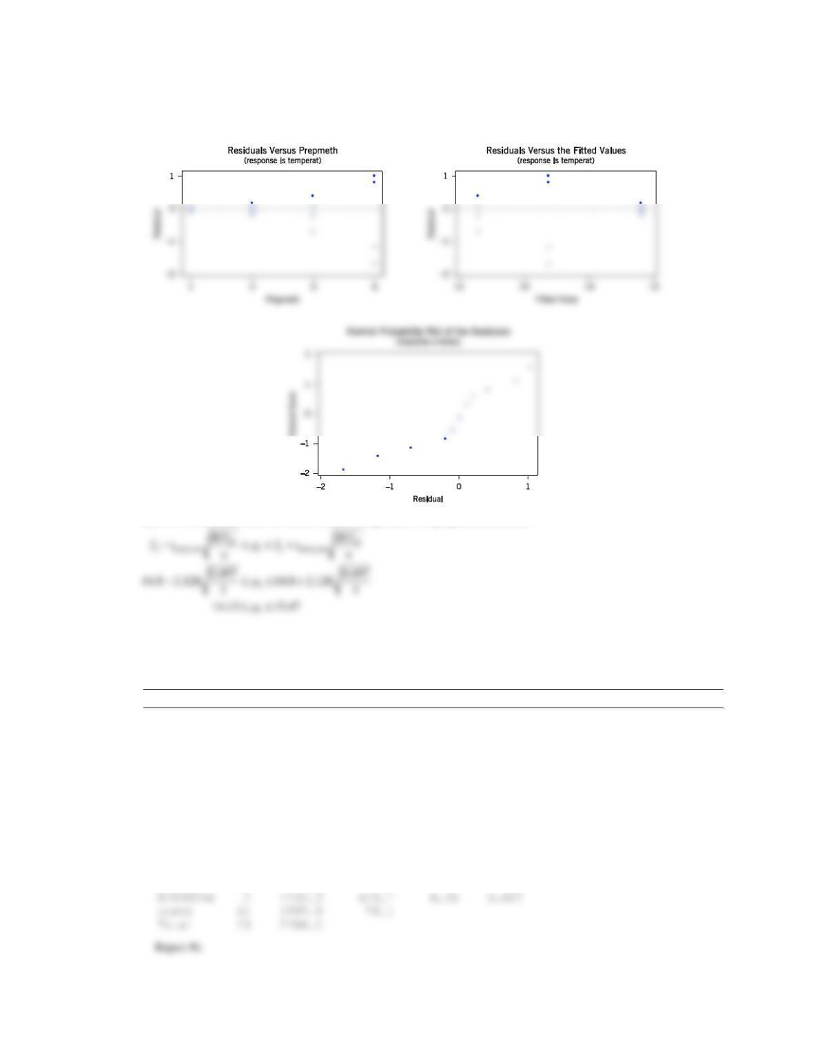
(c) Analyze the residuals from this experiment.
(d) Find a 95% confidence interval on mean Tc when method 1is used to prepare the material.
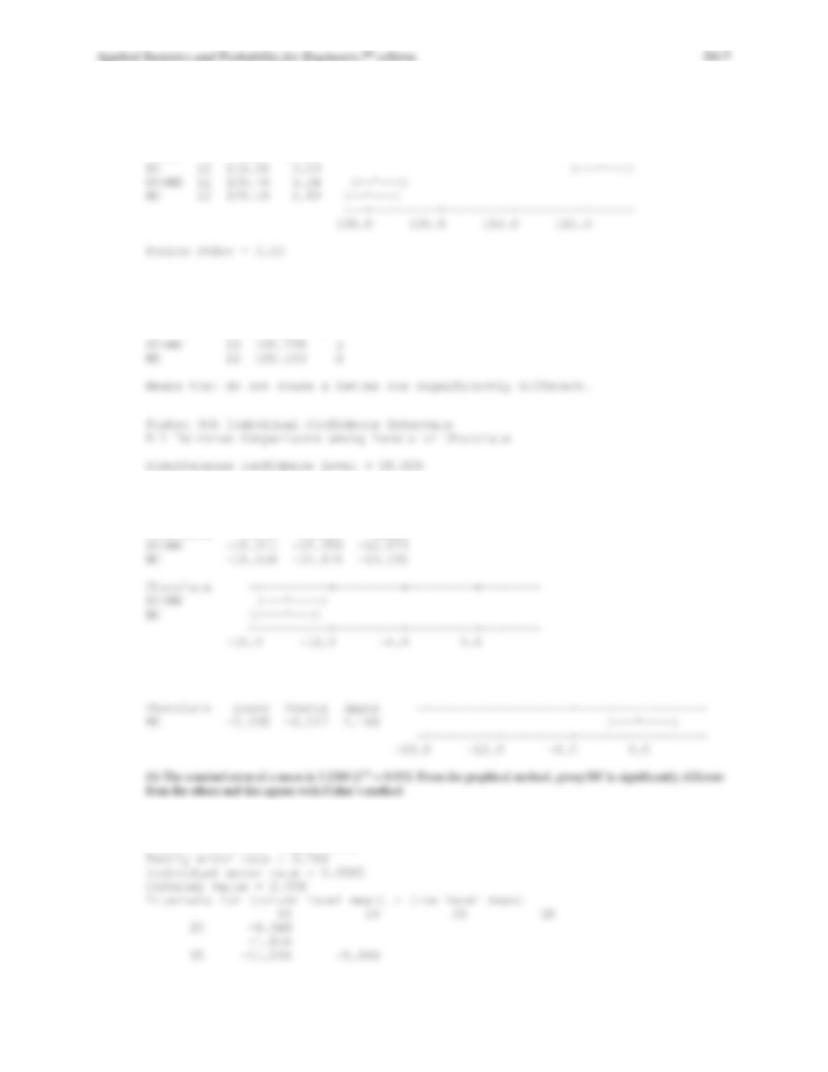
(a) Analysis of Variance of PREPARATION METHOD
Source DF SS MS F P
Applied Statistics and Probability for Engineers,7th edition 2017
13-9
(c) There are some differences in the amount variability at the different preparation methods and there is some
curvature in the normal probability plot. There are also some potential problems with the constant variance assumption
apparent in the fitted value plot.
(d) 95% Confidence interval on the mean of temperature for preparation method 1
13.2.9 A paper in the Journal of the Association of Asphalt Paving Technologists (1990, Vol. 59) described an experiment to
determine the effect of air voids on percentage retained strength of asphalt. For purposes of the experiment, air voids
are controlled at three levels; low (2–4%), medium (4–6%), and high (6–8%). The data are shown in the following
table.
Air Voids
Retained Strength (%)
Low
106
90
103
90
79
88
92
95
Medium
80
69
94
91
70
83
87
83
High
78
80
62
69
76
85
69
85
(a) Do the different levels of air voids significantly affect mean retained strength? Use
= 0.01.
(b) Find the P-value for the F-statistic in part (a).
(c) Analyze the residuals from this experiment.
(d) Find a 95% confidence interval on mean retained strength where there is a high level of air voids.
(e) Find a 95% confidence interval on the difference in mean retained strength at the low and high levels of air voids.
(a) Analysis of Variance for STRENGTH
Source DF SS MS F P
Applied Statistics and Probability for Engineers,7th edition 2017
13–10
(d) 95% Confidence interval on the mean of retained strength where there is a high level of air voids
− +
3 0.025,21 3 0.015,21
EE
i
M S M S
y t y t
nn
13.2.10 An article in Quality Engineering [“Estimating Sources of Variation: A Case Study from Polyurethane Product
Research” (1999–2000, Vol. 12, pp. 89–96)] reported a study on the effects of additives on final polymer properties. In
this case, polyurethane additives were referred to as cross-linkers. The average domain spacing was the measurement of
the polymer property. The data are as follows:
Cross-Linker
Level
Domain Spacing (nm)
−1
8.2
8
8.2
7.9
8.1
8
−0.75
8.3
8.4
8.3
8.2
8.3
8.1
−0.5
8.9
8.7
8.9
8.4
8.3
8.5
0
8.5
8.7
8.7
8.7
8.8
8.8
0.5
8.8
9.1
9.0
8.7
8.9
8.5
1
8.6
8.5
8.6
8.7
8.8
8.8
Applied Statistics and Probability for Engineers,7th edition 2017
13–11
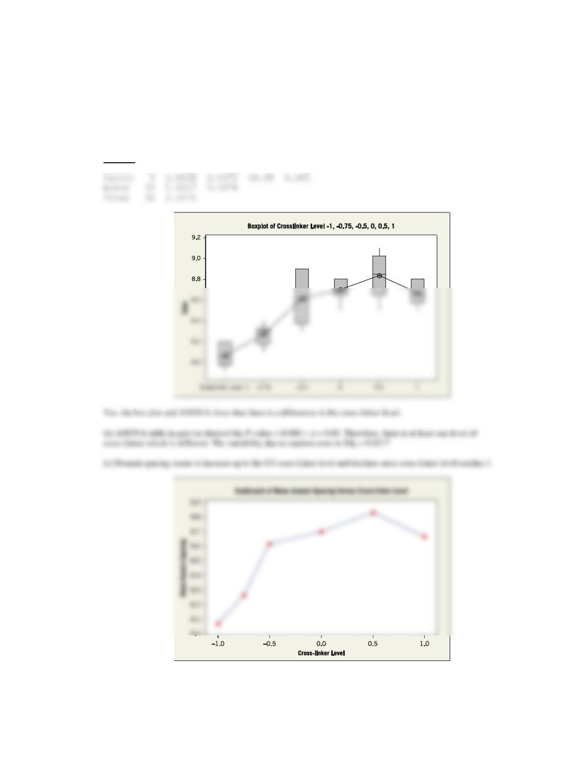
(a) Is there a difference in the cross-linker level? Draw comparative box plots and perform an analysis of variance. Use
= 0.05.
(b) Find the P-value of the test. Estimate the variability due to random error.
(c) Plot average domain spacing against cross-linker level and interpret the results.
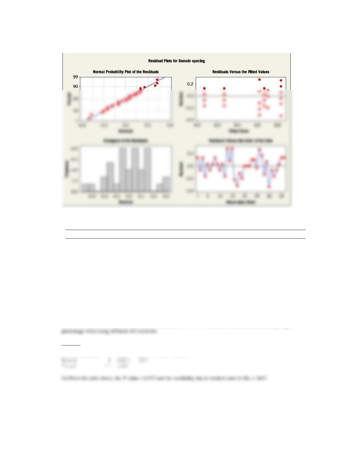
(d) Analyze the residuals from this experiment and comment on model adequacy.
(a)
ANOVA
Source DF SS MS F P
Applied Statistics and Probability for Engineers,7th edition 2017
13–12
(d) The normal probability plot and the residual plots show that the model assumptions are reasonable.
13.2.11 An article in Journal of Food Science [2001, Vol. 66(3), pp. 472–477] reported on a study of potato spoilage based on
different conditions of acidified oxine (AO), which is a mixture of chlorite and chlorine dioxide. The data follow:
AO Solution (ppm)
% Spoilage
50
100
50
60
100
60
30
30
200
60
50
29
400
25
30
15
(a) Do the AO solutions differ in the spoilage percentage? Use
= 0.05.
(b) Find the P-value of the test. Estimate the variability due to random error.
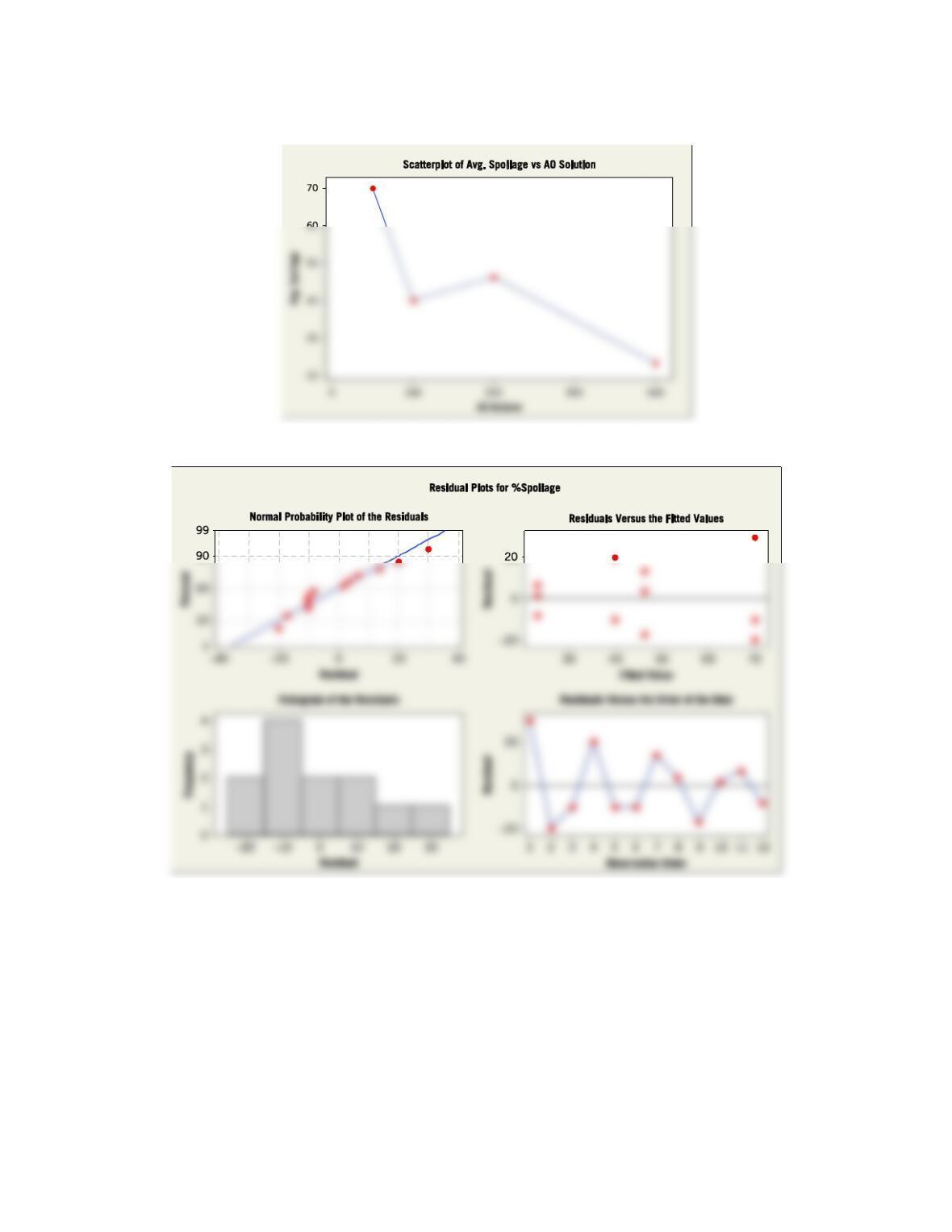
(c) Plot average spoilage against AO solution and interpret the results. Which AO solution would you recommend for
use in practice?
(d) Analyze the residuals from this experiment.
(a) From the analysis of variance shown below, F0.05,3,8 = 4.07 > F0 = 3.43 there is no difference in the spoilage
ANOVA
Source DF SS MS F P
AO solutions 3 3364 1121 3.43 0.073
Applied Statistics and Probability for Engineers,7th edition 2017
13–13
(c) A 400 ppm AO solution should be used because it produces the lowest average spoilage percentage.
(d) The normal probability plot and the residual plots show that the model assumptions are reasonable.
3.2.12 An article in ScientiaIranica [“Tuning the Parameters of an Artificial Neural Network (ANN) Using Central Composite
Design and Genetic Algorithm” (2011, Vol. 18(6), pp. 1600–608)], described a series of experiments
to tune parameters in artificial neural networks. One experiment considered the relationship between model fitness
[measured by the square root of mean square error (RMSE) on a separate test set of data] and model complexity that
were controlled by the number of nodes in the two hidden layers. The following data table (extracted from a much
larger data set) contains three different ANNs: ANN1 has 33 nodes in layer 1 and 30 nodes in layer 2, ANN2 has 49
nodes in layer 1 and 45 nodes in layer 2, and ANN3 has 17 nodes in layer 1 and 15 nodes in layer 2.
Applied Statistics and Probability for Engineers,7th edition 2017
13–14
ANN type
RMSE
ANN1
0.0121
0.0132
0.0011
0.0023
0.0391
0.0054
0.0003
0.0014
ANN2
0.0031
0.0006
0
0
0.022
0.0019
0.0007
0
ANN3
0.1562
0.2227
0.0953
0.8911
1.3892
0.0154
1.7916
0.1992
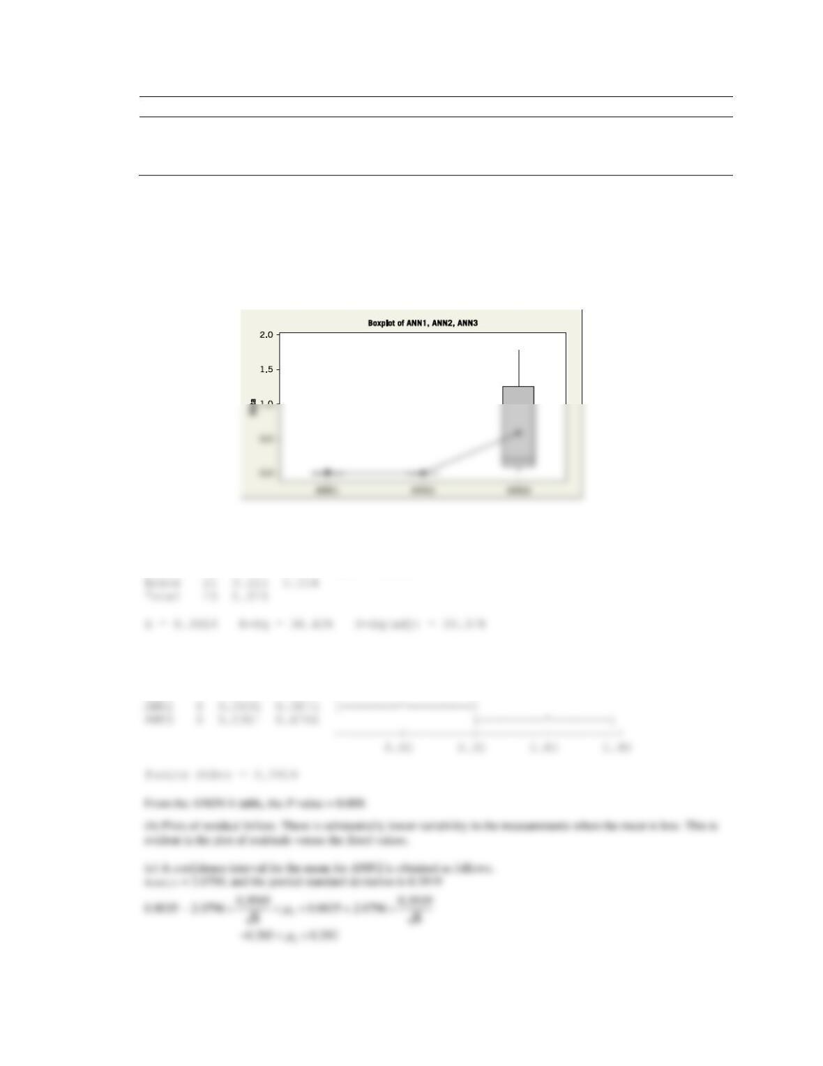
(a) Construct a box plot to compare the different ANNs.
(b) Perform the analysis of variance with
= 0.05. What is the P-value?
(c) Analyze the residuals from the experiment.
(d) Calculate a 95% confidence interval on RMSE for ANN2.
(a)
One-way ANOVA: ANN1, ANN2, ANN3
Source DF SS MS F P
Factor 2 1.848 0.924 6.02 0.009
Individual 95% CIs For Mean Based on
Pooled StDev
Level N Mean StDev ———+———+———+———+
ANN1 8 0.0094 0.0130 (——–*———)
Applied Statistics and Probability for Engineers,7th edition 2017
However, because the variance differs between the ANNs, one might use only the data from ANN2 to construct a
confidence interval. Then,
13.2.13 to 13.2.18 For each of the following exercises, use the previous data to complete these parts.
13.2.13 Chocolate type in Exercise 13.2.3. Use
= 0.05.
(a)
Source DF SS MS F P
13–16
S = 3.230 R-Sq = 85.01% R-Sq(adj) = 84.10%
Individual 95% CIs For Mean Based on
Pooled StDev
Level N Mean StDev —+———+———+———+——
Grouping Information Using Fisher Method
Chocolate N Mean Grouping
DC 12 116.058 A
Chocolate = DC subtracted from:
Chocolate Lower Center Upper
Chocolate = DC+MK subtracted from:
13.2.14 Cotton percentage in Exercise 13.2.4. Use
= 0.05.
Fisher’s pairwise comparisons

Applied Statistics and Probability for Engineers,7th edition 2017
13–17
Applied Statistics and Probability for Engineers,7th edition 2017
13.2.15 Flow rate in Exercise 13.2.5. Use
= 0.01.
Intervals for (column level mean) – (row level mean)
125 160
13.2.16 Preparation method in Exercise 13.2.8. Use
= 0.05.
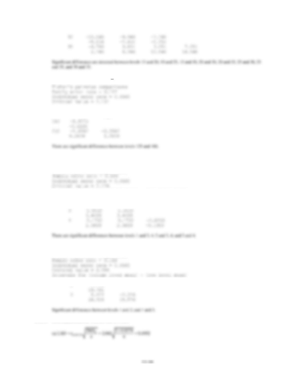
Fisher’s pairwise comparisons
Intervals for (column level mean) – (row level mean)
1 2 3
2 -0.9450
0.9450
13.2.17 Air voids in Exercise 13.2.9. Use
= 0.05.
Fisher’s pairwise comparisons
1 2
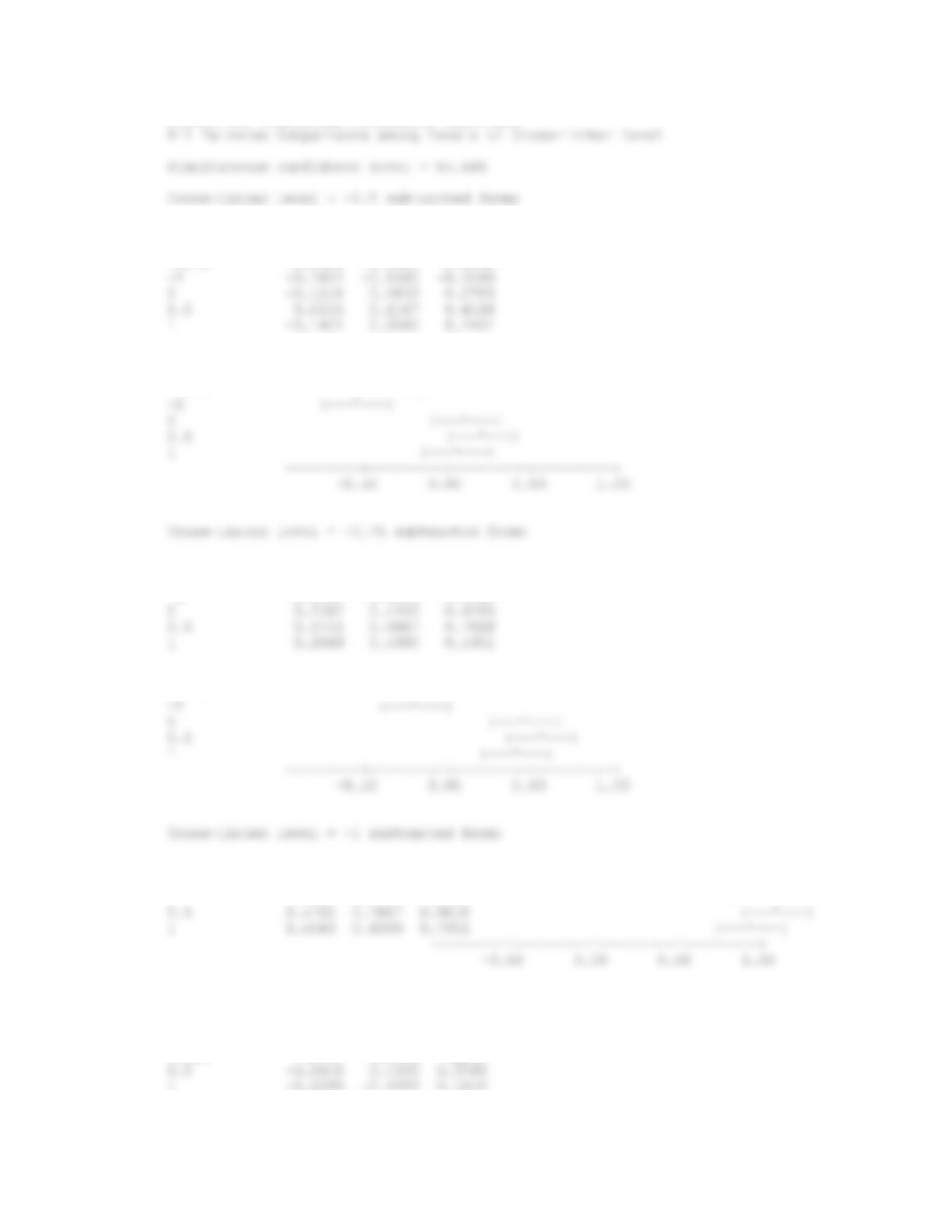
13.2.18 Cross-linker Exercise 13.2.10. Use
= 0.05.

13–19
Applied Statistics and Probability for Engineers,7th edition 2017
13–20
Fisher 95% Individual Confidence Intervals
Cross-linker
level Lower Center Upper
-0.75 -0.5451 -0.3500 -0.1549
Cross-linker
level ———+———+———+———+
-0.75 (—*—)
Cross-linker
level Lower Center Upper
-1 -0.3951 -0.2000 -0.0049
Cross-linker
level ———+———+———+———+
Cross-linker
level Lower Center Upper ———+———+———+———+
0 0.4382 0.6333 0.8285 (—*—)
Cross-linker level = 0 subtracted from:
Cross-linker
level Lower Center Upper