Unlock document.
This document is partially blurred.
Unlock all pages and 1 million more documents.
Get Access
Reserve Problems Chapter 12 Section 2 Problem 3
You have fit a regression model with three regressors to a data set that has 19 observations. The
total sum of squares is 1150 and the model sum of squares is 550.
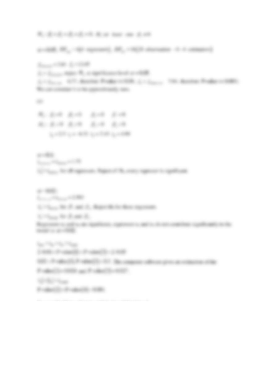
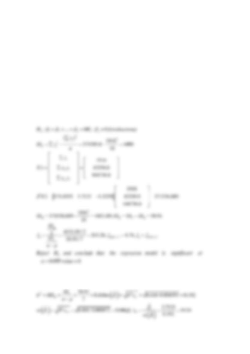
(a) What is the value of R2 for this model? What is the adjusted R2 for this model?
(b) What is the value of the F-statistic and P-value for testing the significance of regression?
What conclusions would you draw about this model if
0.05
=
? What if
0.01
=
?
(c) Suppose that you add two regressors to the model and as a result, the model sum of squares is
now 797. Does it seem to you that adding this factor has improved the model? Use
0.05
=
and
0.025
=
.
SOLUTION
(a)
(b)
(c)
After adding the fourth and fifth regressors:
Reserve Problems Chapter 12 Section 2 Problem 4
Rusting of steel slabs is investigated. Data for the corrosion rate are shown in the following
table.
Temperature,
C°
Humidity,
%
Trace gases in air,
μg/m3
Dust in air,
μg/m3
Corrosion rate, mg/m2
per day
27
49
79
34
157
10
28
59
98
181
0
50
82
53
302
21
30
64
27
90
20
27
65
94
213
29
48
55
51
162
25
41
88
18
159
2
26
86
45
154
26
48
52
99
229
25
47
61
18
149
1
36
51
79
227
12
42
68
36
129
2
50
60
88
282
13
34
70
62
169
4
47
65
87
204
28
25
83
52
132
(a) Fit a multiple linear regression model to these data. Enter negative coefficients as negative
numbers. What are the test statistic and P-value for this regression?
(b) Construct a t-test for each regression coefficient and find the P-values. Which regressors are
significant at
0.09
=
and
0.05
=
?
(c) Fit a new regression model to the corrosion as response using only those regressors
significant at
0.09
=
.
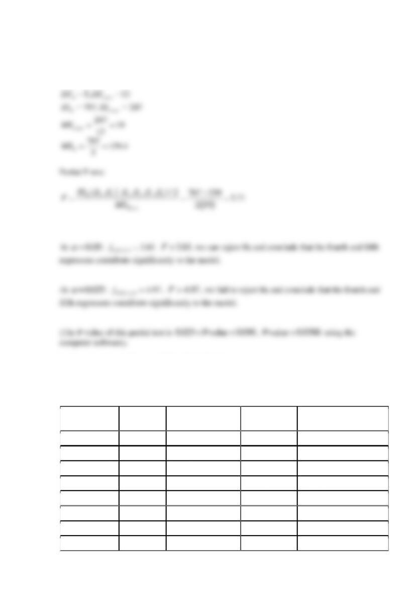
SOLUTION
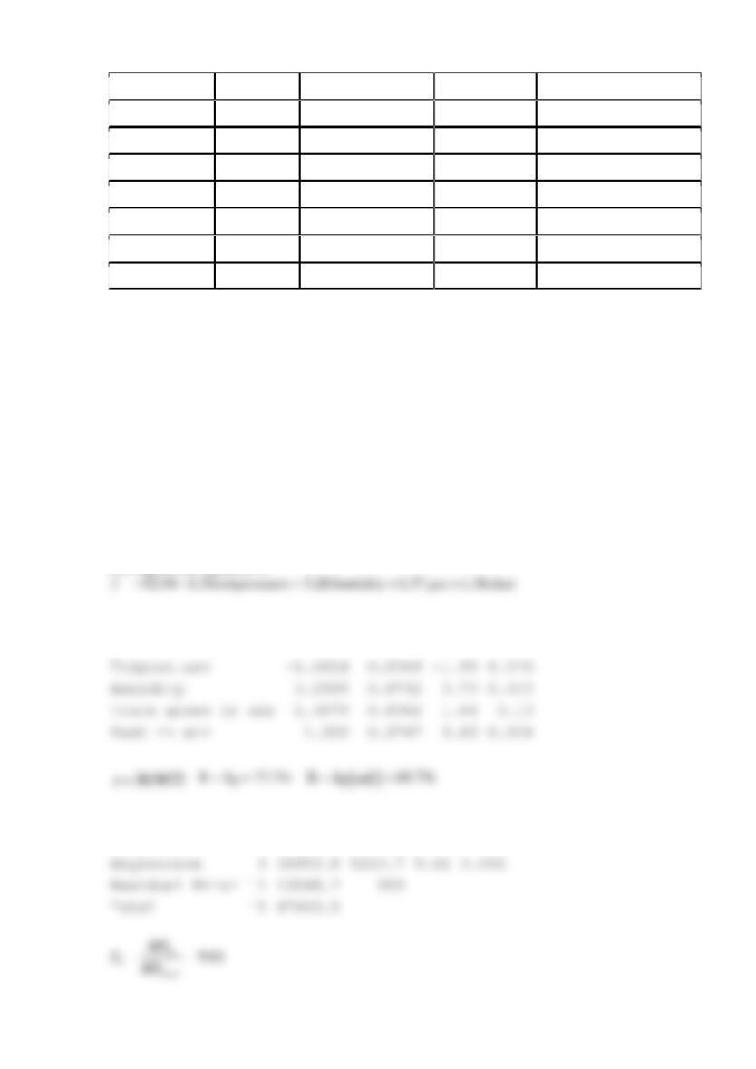
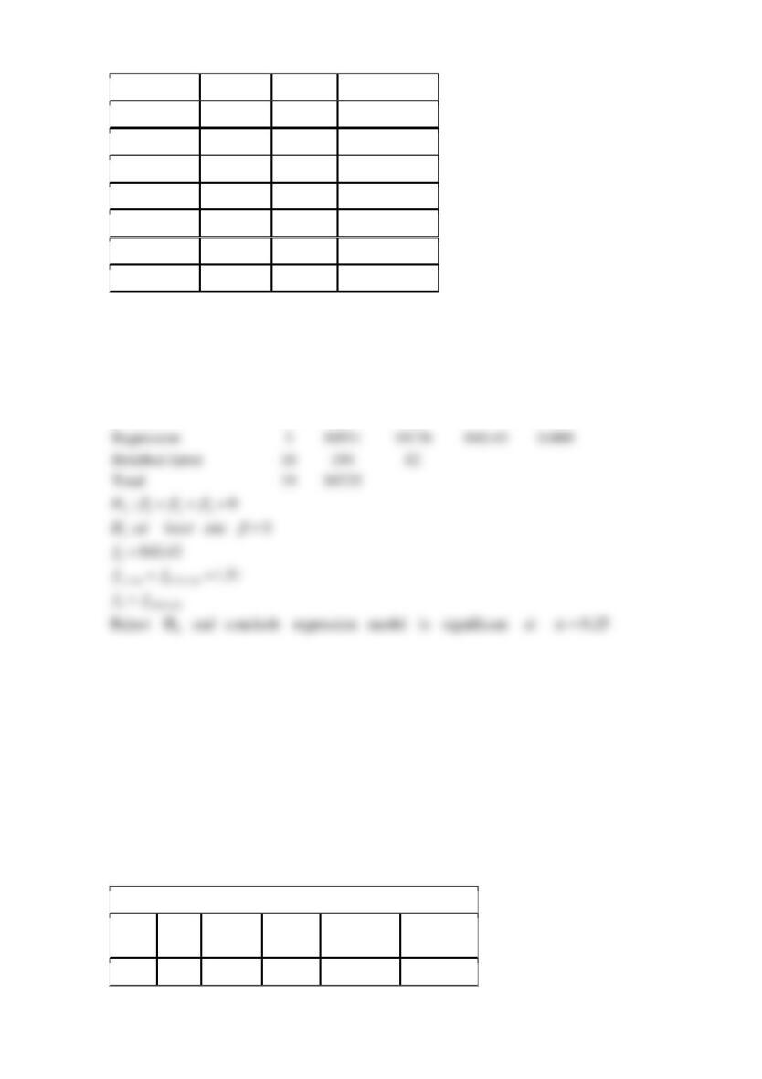
(a)
The regression equation is
Predictor
Coef
SE Coef
T
P
Constant
-92.94
93.73
-0.99
0.343
Analysis of Variance
Source
DF
SS
MS
F
P
(b)
0:H
10
=
20
=
30
=
40
=
0.09:
=
/2, 0.045,11 1.86
np
tt
−==
0.05:
=
0 0.025,11
The regression equation is
43.29 1.9 2.83 0.99
ˆ
y temperature humidity dust= − + +
Predictor
Coef
SE Coef
T
P
Constant
43.29
45.9
0.94
0.364
Reserve Problems Chapter 12 Section 2 Problem 5
A class of 64 students has two hourly exams and a final exam.
The following are some quantities of interest:
( ) ( )
1
0.912917 9.82 03 7.11 04 4871.0
0.00982 1.5 04 4.16 05 426011.0
0.000711 4.16 05 5.81 05 367576.5
ee
X X e e X y
ee
−
− − − −
= − − − − =
− − − −
Assume
2
1
64
411222.7041
i
i
y y y
=
= =
(a) Test the hypotheses that each of the slopes is zero.
1. Round your answer to two decimal places.
2. Round your answer to two decimal places.
3. Round your answers to four decimal places.
4. Round your answers to two decimal places.
5.
64,n=
so degrees of freedom:
6. Round your answers to three decimal places.
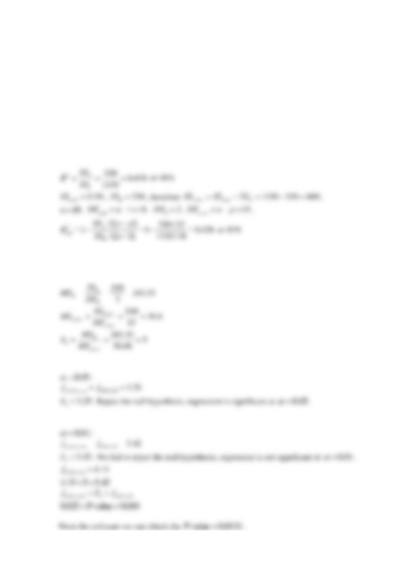
(b) What is the value of
2
R
for this model?
(c) What is the residual standard deviation?
(d) Do you believe that the professor can predict the final grade well enough from the two hourly
tests to consider not giving the final exam?
SOLUTION
(a)
1.
( )
1411222.7041 403874.0241 7348.68SSE y y y X X X X y
−
= − = − =
Reserve Problems Chapter 12 Section 2 Problem 6
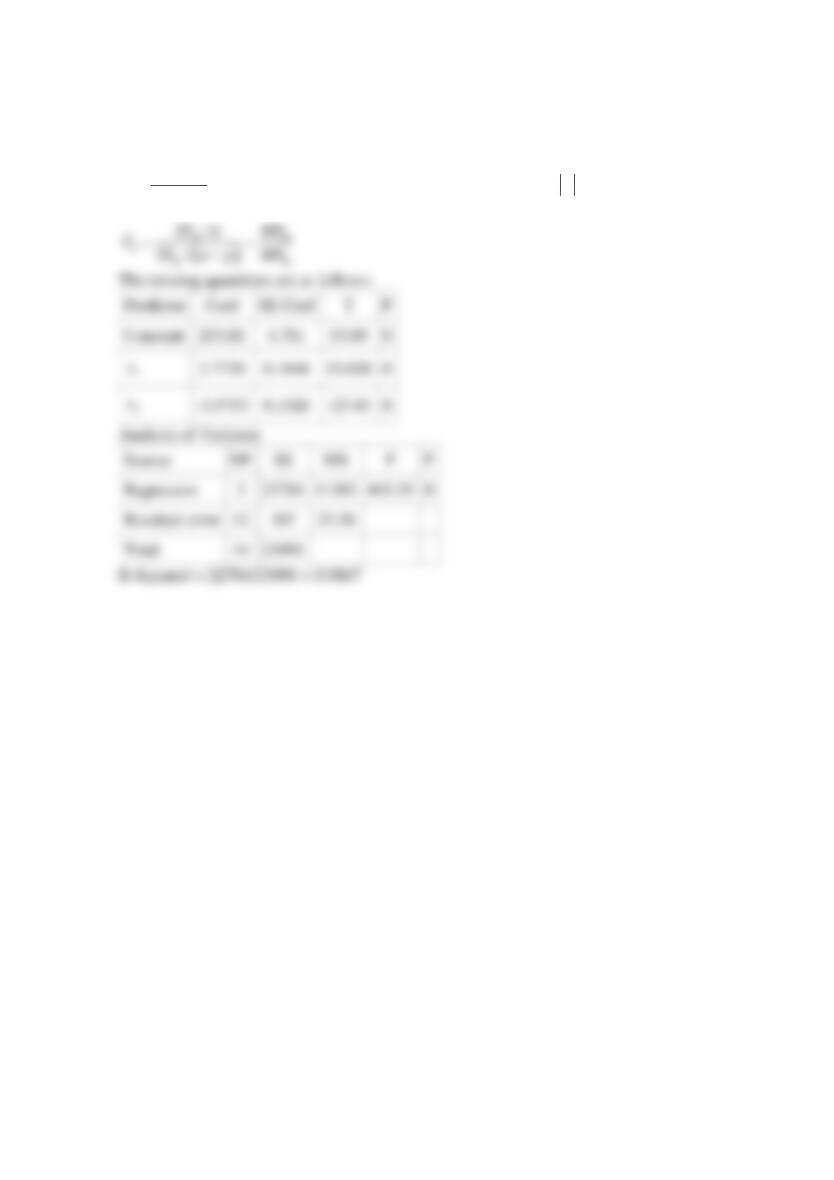
Consider the following computer output.
The regression equation is
( )
12
254 2.77 3 8
ˆ.5y x x= + + −
.
Fill in the missing quantities.
Predictor
Coef
SE Coef
T
P
Constant
254.026
4.942
1
x
2.8641
0.1952
14.673
2
x
-3.8141
0.1672
S=5.05756 R-Sq=? R-Sq(adj)=98.4%
Analysis of Variance
Source
DF
SS
MS
F
P
Regression
2
22784
11392
Residual error
Total
14
23091
SOLUTION
( )
0
0
ˆ
ˆ
jj
j
t
se
−
=
, null hypothesis
0jj
=
is rejected at
level if
0 /2,np
tt
−
Reserve Problems Chapter 12 Section 2 Problem 7
A study was performed to investigate the shear strength of soil (y) as it related to depth in feet (
1
x
) and percent of moisture content (
2
x
). Ten observations were collected, and the following
summary quantities obtained:
10n=
,
1223
i
x=
,
2553
i
x=
,
1916
i
y=
,
2
15202.4
i
x=
,
2
231729
i
x=
,
12
12352
ii
xx=
,
143550.8
ii
xy=
,
2104736.8
ii
xy=
, and
2371595.6
i
y=
. Consider the regression model fit to the soil shear strength data.
Use the values of regression coefficients rounded at least to four decimal places in your
calculations to obtain the answers.
(a) Test for significance of regression using
0.05
=
. What is the P-value?
1. Round your answer to the nearest integer.
2. Round your answers to two decimal places.
3. Round your answer to two decimal places.
4. ______
0
H
at
0.05
=
.
(b) Construct the t-test on each regression coefficient. Calculate P-values.
1. Round your answers to three decimal places.
2. Round your answers to three decimal places.
3.
1:
_____
0
H
at
0.05
=
.
SOLUTION
(a)
10n=
,
2k=
,
3p=
,
0.05
=
(b)

Reserve Problems Chapter 12 Section 2 Problem 8
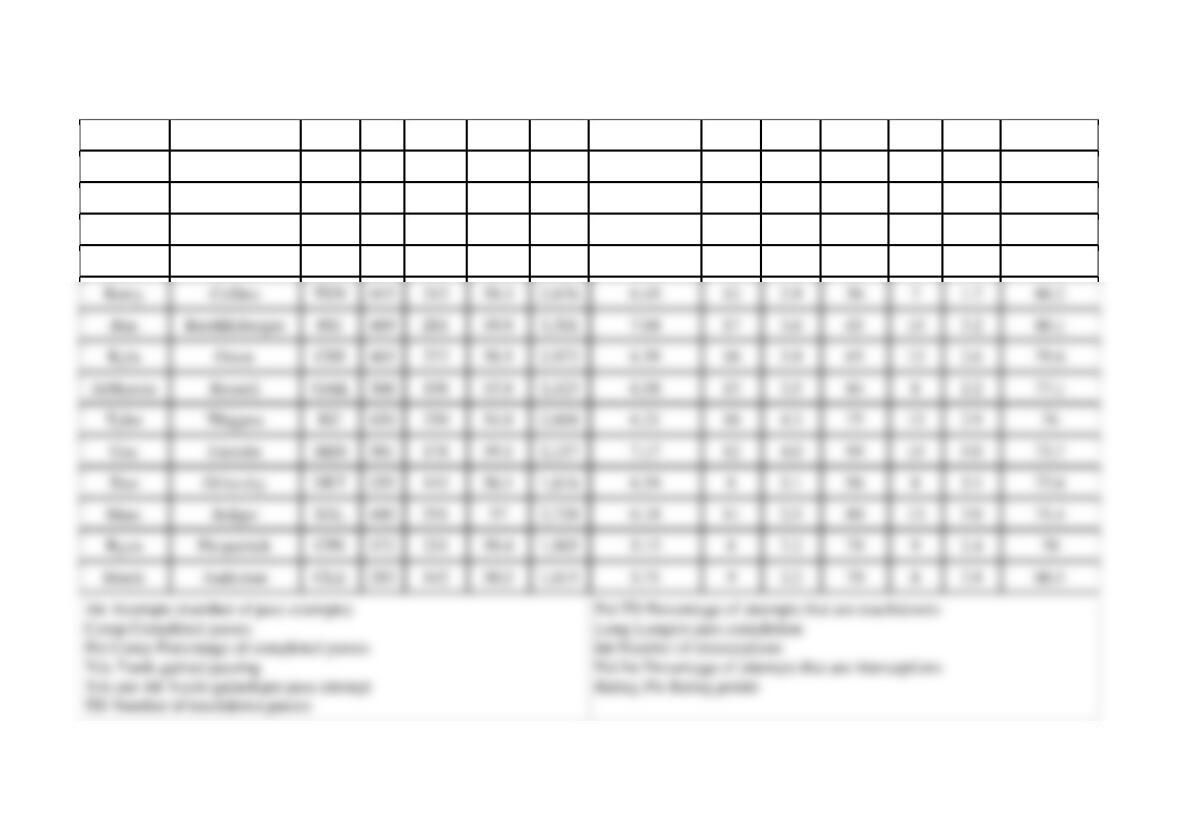
Table provides the highway gasoline mileage test results for 2005 model year vehicles from
DaimlerChrysler. The full table of data (available on the book’s Web site) contains the same data
for 2005 models from over 250 vehicles from many manufacturers (Environmental Protection Agency
Web site www.epa.gov/otaq/cert/mpg/testcars/database). . Consider the gasoline mileage data.
Table DaimlerChrysler Fuel Economy and Emissions
mfr
carline
car/truck
cid
rhp
trns
drv
od
etw
cmp
axle
n/v
a/c
hc
co
co2
mpg
20
300C/SRT-8
C
215
253
L5
4
2
4500
9.9
3.07
30.9
Y
0.011
0.09
288
30.8
20
CARAVAN 2WD
C
201
180
L4
F
2
4500
9.3
2.49
32.3
Y
0.014
0.11
274
32.5
20
CROSSFIRE ROADSTER
C
196
168
L5
R
2
3375
10
3.27
37.1
Y
0.001
0.02
250
35.4
20
DAKOTA PICKUP 2WD
C
226
210
L4
R
2
4500
9.2
3.55
29.6
Y
0.012
0.04
316
28.1
20
DAKOTA PICKUP 4WD
C
226
210
L4
4
2
5000
9.2
3.55
29.6
Y
0.011
0.05
365
24.4
20
DURANGO 2WD
C
348
345
L5
R
2
5250
8.6
3.55
27.2
Y
0.023
0.15
367
24.1
20
GRAND CHEROKEE 2WD
C
226
210
L4
R
2
4500
9.2
3.07
30.4
Y
0.006
0.09
312
28.5
20
GRAND CHEROKEE 4WD
C
348
230
L5
4
2
5000
9
3.07
24.7
Y
0.008
0.11
369
24.2
20
LIBERTY/CHEROKEE 2WD
C
148
150
M6
R
2
4000
9.5
4.1
41
Y
0.004
0.41
270
32.8
20
LIBERTY/CHEROKEE 4WD
C
226
210
L4
4
2
4250
9.2
3.73
31.2
Y
0.003
0.04
317
28
20
NEON/SRT-4/SX 2.0
C
122
132
L4
F
2
3000
9.8
2.69
39.2
Y
0.003
0.16
214
41.3
20
PACIFICA 2WD
C
215
249
L4
F
2
4750
9.9
2.95
35.3
Y
0.022
0.01
295
30
20
PACIFICA AWD
C
215
249
L4
4
2
5000
9.9
2.95
35.3
Y
0.024
0.05
314
28.2
20
PT CRUISER
C
148
220
L4
F
2
3625
9.5
2.69
37.3
Y
0.002
0.03
260
34.1
20
RAM 1500 PICKUP 2WD
C
500
500
M6
R
2
5250
9.6
4.1
22.3
Y
0.01
0.1
474
18.7
20
RAM 1500 PICKUP 4WD
C
348
345
L5
4
2
6000
8.6
3.92
29
Y
0
0
0
20.3
20
SEBRING 4-DR
C
165
200
L4
F
2
3625
9.7
2.69
36.8
Y
0.011
0.12
252
35.1
20
STRATUS 4-DR
C
148
167
L4
F
2
3500
9.5
2.69
36.8
Y
0.002
0.06
233
37.9
20
TOWN & COUNTRY 2WD
C
148
150
L4
F
2
4250
9.4
2.69
34.9
Y
0
0.09
262
33.8
20
VIPER CONVERTIBLE
C
500
501
M6
R
2
3750
9.6
3.07
19.4
Y
0.007
0.05
342
25.9
20
WRANGLER/TJ 4WD
C
148
150
M6
4
2
3625
9.5
3.73
40.1
Y
0.004
0.43
337
26.4
mfr-mfr code
carline-car line name (test vehicle model name)
car/truck-‘C’ for passenger vehicle and ‘T’ for truck
cid-cubic inch displacement of test vehicle
rhp-rated horsepower
trns-transmission code
drv-drive system code
od-overdrive code
etw-equivalent test weight
cmp-compression ratio
axle-axle ratio
n/v-n/v ratio (engine speed versus vehicle speed at 50 mph)
a/c-indicates air conditioning simulation
hc-HC(hydrocarbon emissions) Test level composite results
co-CO(carbon monoxide emissions) Test level composite results
co2-CO2(carbon dioxide emissions) Test level composite results
mpg-mpg(fuel economy, miles per gallon)
Fit a linear regression model to these data to estimate gasoline mileage that uses the following regressors: cid, rhp, etw, cmp, axle, n/v.
(a) Test for significance of regression using
0.025
=
.
(b) Find the t-test statistic for each regressor (for
1
through
6
).
SOLUTION
(a)
0123456
:0H
= = = = = =
(b)
49.90 0.01045 0.001204 0.003236 0.2924 3.855 0.189
ˆ7y x x x x x x= − − − + − +
Reserve Problems Chapter 12 Section 2 Problem 9
An engineer at a semiconductor company wants to model the relationship between the device
HFE (y) and three parameters: Emitter-RS (
1
x
), Base-RS (
2
x
), and Emitter-to-Base RS (
3
x
).
The data are shown in the table.
Table Semiconductor Data.
x1
Emitter-RS
x2
Base-RS
x3
E-B-RS
y
HFE-1M-5V
14.62
226
7
128.4
15.63
220
3.375
52.62
14.62
217.4
6.375
113.9
15
220
6
98.01
14.5
226.5
7.625
139.9
15.25
224.1
6
102.6
16.12
220.5
3.375
48.14
15.13
223.5
6.125
109.6
15.5
217.6
5
82.68
15.13
228.5
6.625
112.6
15.5
230.2
5.75
97.52
16.12
226.5
3.75
59.06
15.13
226.6
6.125
111.8
15.63
225.6
5.375
89.09
15.38
229.7
5.875
101
14.38
234
8.875
171.9
15.5
230
4
66.8
14.25
224.3
8
157.1
14.5
240.5
10.87
208.4
14.62
223.7
7.375
133.4
Test for significance of regression using α = 0.25.
SOLUTION
Analysis of Variance
Source
DF
SS
MS
F
P
Reserve Problems Chapter 12 Section 2 Problem 10
An article in Cancer Epidemiology, Biomarkers and Prevention (1996, Vol. 5, pp. 849–852)
reported on a pilot study to assess the use of toenail arsenic concentrations as an indicator of
ingestion of arsenic-containing water. Twenty-one participants were interviewed regarding use
of their private (unregulated) wells for drinking and cooking, and each provided a sample of
water and toenail clippings. Table E12-8 showed the data of age (years), sex of person (1 = male, 2 =
female), proportion of times household well used for drinking (1 ≤ 1/4, 2 = 1/4, 3 = 1/2, 4 = 3/4,
5 ≥ 3/4), proportion of times household well used for cooking (1 ≤1/4, 2 = 1/4, 3 = 1/2, 4 = 3/4,
5 ≥ 3/4), arsenic in water (ppm), and arsenic in toenails (ppm) respectively.
Consider the regression model fit to the arsenic data. Use arsenic in nails as the response and
age, drink use, and cook use as the regressors.
Table Arsenic Data
Age
Sex
Drink
Use
Cook
Use
Arsenic
Water
Arsenic
Nails
44
2
5
5
0.00087
0.119
45
2
4
5
0.00021
0.118
44
1
5
5
0
0.099
66
2
3
5
0.00115
0.118
37
1
2
5
0
0.277
45
2
5
5
0
0.358
47
1
5
5
0.00013
0.08
38
2
4
5
0.00069
0.158
41
2
3
2
0.00039
0.31
49
2
4
5
0
0.105
72
2
5
5
0
0.073
45
2
1
5
0.046
0.832
53
1
5
5
0.0194
0.517
86
2
5
5
0.137
2.252
8
2
5
5
0.0214
0.851
32
2
5
5
0.0175
0.269
44
1
5
5
0.0764
0.433
63
2
5
5
0
0.141
42
1
5
5
0.0165
0.275
62
1
5
5
0.00012
0.135
36
1
5
5
0.0041
0.175
(a) Test for significance of regression using
0.05
=
. What is the P-value for this test? Round
your answers to two decimal places.
(b) Construct a t-test on each regression coefficient. Use
0.05
=
.
1. For
1
:
2. For
2
:
3. For
3
:
SOLUTION
(a)
Analysis of Variance
Source
DF
SS
MS
F
P
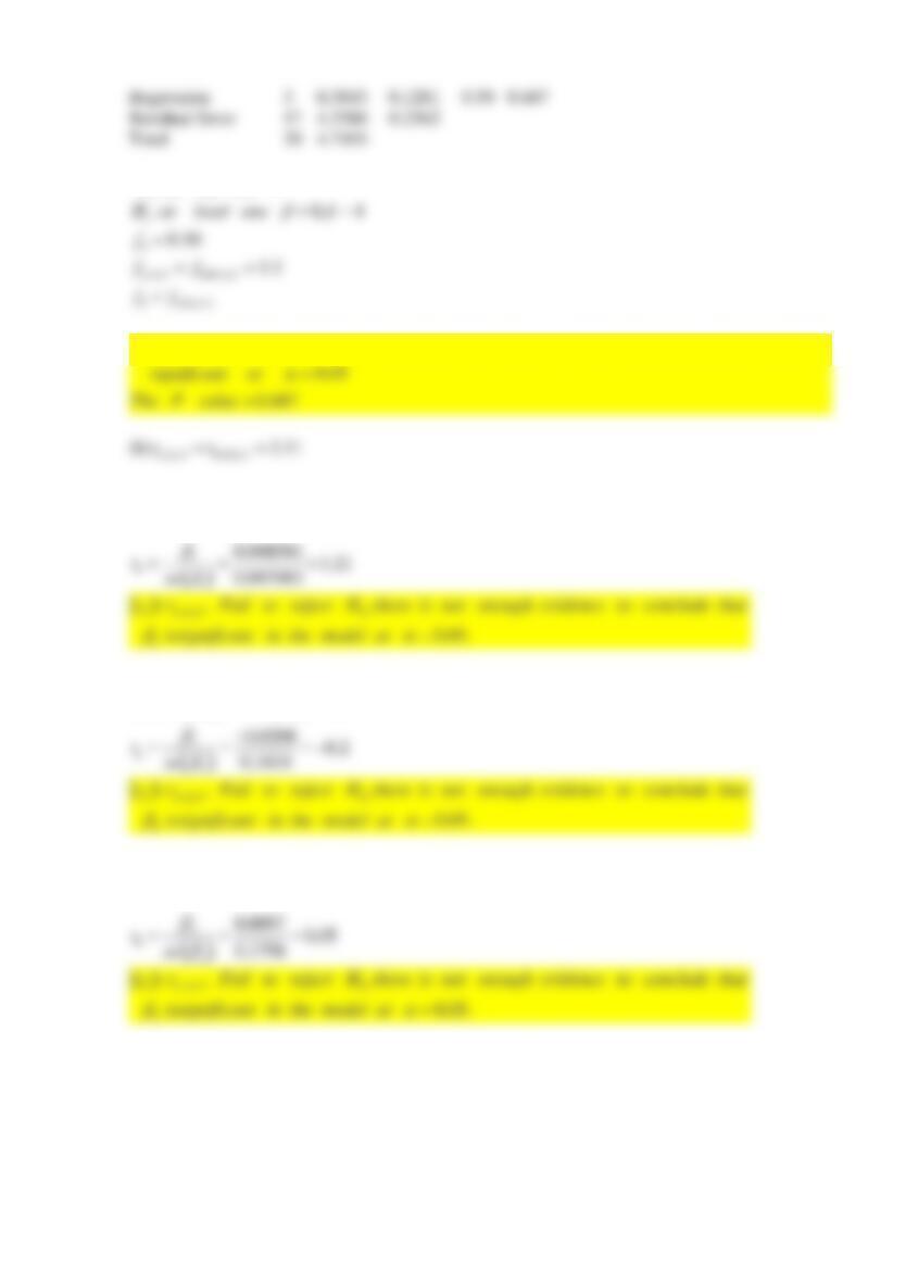
0 1 2 3
:0H
= = =
0.
Fail to reject H There is insufficient evidence to conclude that the model is
(b.1)
0 1 1 1
: 0; : 0; 0.05HH
= =
(b.2)
0 2 1 2
: 0; : 0; 0.05HH
= =
(b.3)
0 3 1 3
: 0; : 0; 0.05HH
= =
Reserve Problems Chapter 12 Section 2 Problem 11
An article in Technometrics (1974, Vol. 16, pp. 523–531) considered the following stack-loss
data from a plant oxidizing ammonia to nitric acid. Twenty-one daily responses of stack loss (the
amount of ammonia escaping) were measured with air flow
1
x
, temperature
2
x
, and acid
concentration
3
x
.
y
1
x
2
x
3
x
42
80
27
89
37
80
27
88
37
75
25
90
28
62
24
87
18
62
22
87
18
62
23
87
19
62
24
93
20
62
24
93
15
58
23
87
14
58
18
80
14
58
18
89
13
58
17
88
11
58
18
82
12
58
19
93
8
50
18
89
7
50
18
86
8
50
19
72
8
50
19
79
9
50
20
80
15
56
20
82
15
70
20
91
Consider the regression model fit to the stack loss data. Use stack loss as the response.
(a) Test for significance of regression using
0.10
=
. What is the P-value for this test?
(b) Construct a t-test on each regression coefficient. Use
0.10
=
.
1. For
1
:
2. For
2
:
3. For
3
:
SOLUTION
(a)
0 1 2 3 1
: 0; : 0; 0.10H H at least one
= = = =
(b.1)
( )
22
1
10.52; 0.1349 0
ˆ
ˆˆ
.13
E jj
MS se c
= = = =
(b.3)
( )
2
30.1563
ˆ0.16
ˆjj
se c
= =
Reserve Problems Chapter 12 Section 2 Problem 12
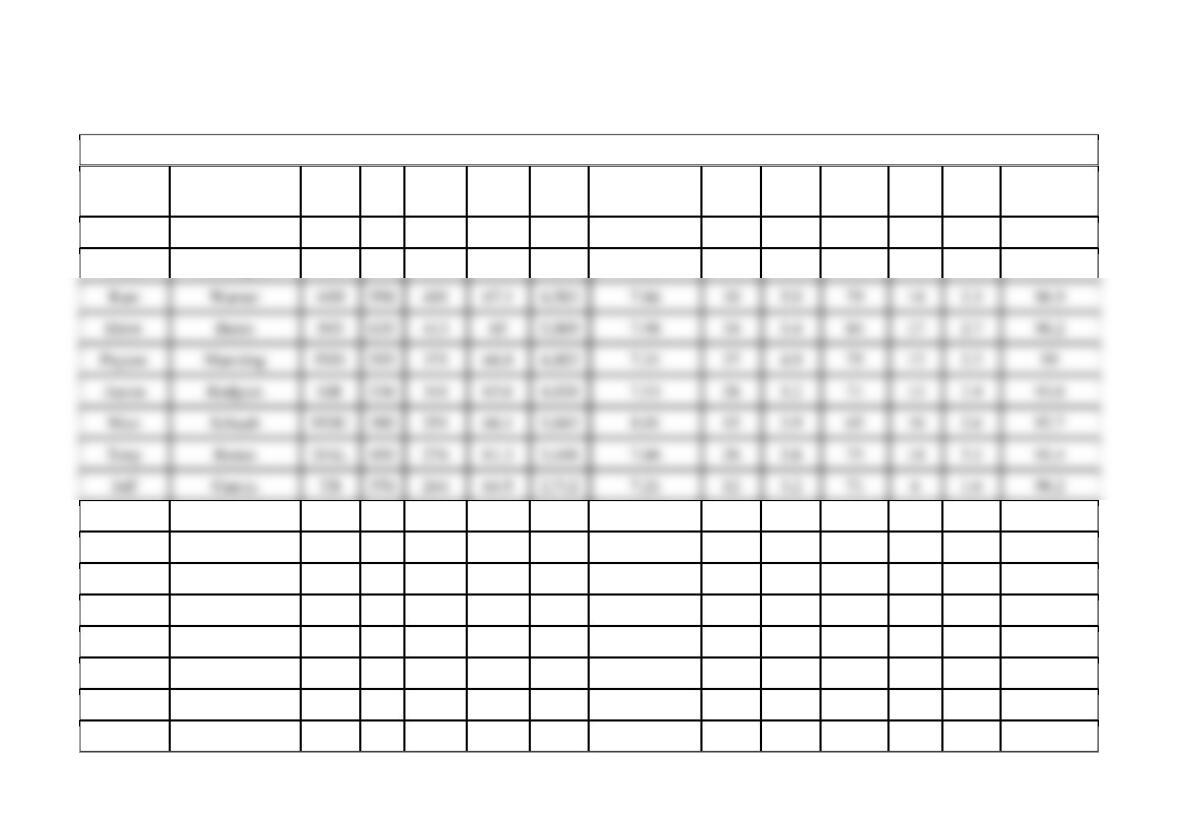
Table presents quarterback ratings for the 2008 National Football League season (The Sports Network).
Table Quarterback Ratings for the 2008 National Football League Season
Player
Team
Att
Comp
Pct
Comp
Yds
Yds per
Att
TD
Pct
TD
Lng
Int
Pct
Int
Rating
Pts
Philip
Rivers
SD
478
312
65.3
4,009
8.39
34
7.1
67
11
2.3
105.5
Chad
Pennington
MIA
476
321
67.4
3,653
7.67
19
4.0
80
7
1.5
97.4
Matt
Cassel
NE
516
327
63.4
3,693
7.16
21
4.1
76
11
2.1
89.4
Matt
Ryan
ATL
434
265
61.1
3,440
7.93
16
3.7
70
11
2.5
87.7
Shaun
Hill
SF
288
181
62.8
2,046
7.1
13
4.5
48
8
2.8
87.5
Seneca
Wallace
SEA
242
141
58.3
1,532
6.33
11
4.5
90
3
1.2
87
Eli
Manning
NYG
479
289
60.3
3,238
6.76
21
4.4
48
10
2.1
86.4
Donovan
McNabb
PHI
571
345
60.4
3,916
6.86
23
4.0
90
11
1.9
86.4
Jay
Cutler
DEN
616
384
62.3
4,526
7.35
25
4.1
93
18
2.9
86
Trent
Edwards
BUF
374
245
65.5
2,699
7.22
11
2.9
65
10
2.7
85.4
Jake
Delhomme
CAR
414
246
59.4
3,288
7.94
15
3.6
65
12
2.9
84.7
Jason
Campbell
WAS
506
315
62.3
3,245
6.41
13
2.6
67
6
1.2
84.3
David
Garrard
JAC
535
335
62.6
3,620
6.77
15
2.8
41
13
2.4
81.7
Brett
Favre
NYJ
522
343
65.7
3,472
6.65
22
4.2
56
22
4.2
81
Joe
Flacco
BAL
428
257
60
2,971
6.94
14
3.3
70
12
2.8
80.3


