(a) What proportion of total variability is explained by this model?
(b) Are there any influential points in these data?
SOLUTION
The regression equation is
Rating Pts 2.99 1.20Pct Comp 4.60Pct TD 3.81Pct Int= + + −
Predictor
Coef
Constant
2.986
Pct Comp
1.19857
0.00706
0.01198
0.00413
0.00465
0.03510
0.00015
0.04000
0.00015
0.00703
0.00054
0.03460
0.00175
0.07326
0.00458
0.00006
0.00086
0.00973
0.07478
0.00899
0.00001
0.44941
0.00268
0.00200
0.00391
0.00710
0.04938
0.02197
0.01702
0.00002
0.00002
0.25999
0.01377
Pct TD
Pct Int
distance greater than 1, two points are different and might be further studied for influence.
Reserve Problems Chapter 12 Section 5 Problem 7
Heat treating is often used to carburize metal parts such as gears. The thickness of the carburized
layer is considered a crucial feature of the gear and contributes to the overall reliability of the
part. Because of the critical nature of this feature, two different lab tests are performed on each
furnace load. One test is run on a sample pin that accompanies each load. The other test is a
destructive test that cross-sections an actual part. This test involves running a carbon analysis on
the surface of both the gear pitch (top of the gear tooth) and the gear root (between the gear
teeth). Table given below shows the results of the pitch carbon analysis test for 32 parts.
The regressors are furnace temperature (TEMP), carbon concentration and duration of the
carburizing cycle (SOAKPCT, SOAKTIME), and carbon concentration and duration of the
diffuse cycle (DIFFPCT, DIFFTIME). The response is the result of the pitch carbon analysis test
(PITCH).
TEMP
SOAKTIME
SOAKPCT
DIFFTIME
DIFFPCT
PITCH
1650
0.58
1.10
0.25
0.90
0.013
1650
0.66
1.10
0.33
0.90
0.035
1650
0.66
1.10
0.33
0.90
0.015
1650
0.66
1.10
0.33
0.95
0.016
1600
0.66
1.15
0.33
1.00
0.015
1600
0.66
1.15
0.33
1.00
0.016
1650
1.00
1.10
0.50
0.80
0.033

1650
1.17
1.10
0.58
0.80
0.021
1650
1.17
1.10
0.58
0.80
0.018
1650
1.17
1.10
0.58
0.80
0.019
1650
1.17
1.10
0.58
0.90
0.040
1650
1.17
1.10
0.58
0.90
0.019
1650
1.17
1.15
0.58
0.90
0.021
1650
1.20
1.15
1.10
0.80
0.025
1650
2.00
1.15
1.00
0.80
0.025
1650
2.00
1.10
1.10
0.80
0.026
1650
2.20
1.10
1.10
0.80
0.024
1650
2.20
1.10
1.10
0.80
0.025
1650
2.20
1.15
1.10
0.80
0.024
1650
2.20
1.10
1.10
0.90
0.025
1650
2.20
1.10
1.10
0.90
0.027
1650
2.20
1.10
1.50
0.90
0.026
1650
3.00
1.15
1.50
0.80
0.029
1650
3.00
1.10
1.50
0.70
0.030
1650
3.00
1.10
1.50
0.75
0.028
1650
3.00
1.15
1.66
0.85
0.032
1650
3.33
1.10
1.50
0.80
0.033
1700
4.00
1.10
1.50
0.70
0.039
1650
4.00
1.10
1.50
0.70
0.040
1650
4.00
1.15
1.50
0.85
0.035
1700
12.50
1.00
1.50
0.70
0.056
1700
18.50
1.00
1.50
0.70
0.030
(a) Calculate the percent of variability explained by this model.
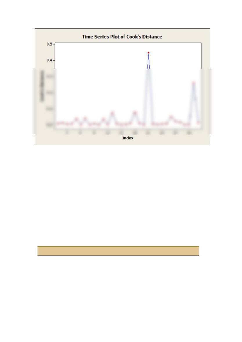
(b) Calculate Cook’s distance for each observation and provide an interpretation of this statistic.
SOLUTION
The regression equation is
Predictor
Coef
Constant
–0.07837
TEMP
4e-005
(b) Cook’s distance values
0.01811
0.00058
0.00191
0.00206
0.02458
0.10379
0.09673
0.01555
0.0061
0.00011
0.01506
8e-005
0.01599
0.00335
0.00102
0.00142
0.00684
0.00122
0.04399
0.00105
0.01499
0.1402
0.04847
0.01505
0.05569
0.00737
0.0094
0.33881
0.44568
0.00947
0.03692
0.86993
Reserve Problems Chapter 12 Section 5 Problem 8
Consider the following stack-loss data from a plant oxidizing ammonia to nitric acid. Twenty-
one daily responses of stack loss (the amount of ammonia escaping) were measured with air flow
1
x
, temperature
2
x
, and acid concentration
3
x
.
y
1
x
2
x
3
x
38
80
27
89
37
80
27
88
41
75
25
90
28
62
24
87
18
62
22
87
18
62
23
87
19
62
24
93
20
62
24
93
19
58
23
87
SOAKTIME
SOAKPCT
DIFFTIME
0.00779
DIFFPCT
–0.00313

14
58
18
80
14
58
18
89
13
58
17
88
11
58
18
82
12
58
19
93
12
50
18
89
7
50
18
86
8
50
19
72
8
50
19
79
9
50
20
80
15
56
20
82
15
70
20
91
(a) What proportion of total variability is explained by this model?
(b) Calculate Cook’s distance for the observations in this data set. Are there any influential
points in these data?
SOLUTION
Predictor
Coef
Constant
-43.5
(b) Cook’s distance values
Cook’s D
0.00
0.02
0.36
0.08

0.13
0.00
0.04
0.00
0.01
0.00
0.50
Reserve Problems Chapter 12 Section 5 Problem 9
Heat treating is often used to carburize metal parts such as gears. The thickness of the carburized
layer is considered a crucial feature of the gear and contributes to the overall reliability of the
part. Because of the critical nature of this feature, two different lab tests are performed on each
furnace load. One test is run on a sample pin that accompanies each load. The other test is a
destructive test that cross-sections an actual part. This test involves running a carbon analysis on
the surface of both the gear pitch (top of the gear tooth) and the gear root (between the gear
teeth). Table given below shows the results of the pitch carbon analysis test for 32 parts.
TEMP
SOAKTIME
SOAKPCT
DIFFTIME
DIFFPCT
PITCH
1650
0.58
1.10
0.25
0.90
0.013
1650
0.66
1.10
0.33
0.90
0.018
1650
0.66
1.10
0.33
0.90
0.015
1650
0.66
1.10
0.33
0.95
0.016
1600
0.66
1.15
0.33
1.00
0.015
1600
0.66
1.15
0.33
1.00
0.016
1650
1.00
1.10
0.50
0.80
0.014
1650
1.17
1.10
0.58
0.80
0.021
1650
1.17
1.10
0.58
0.80
0.018
1650
1.17
1.10
0.58
0.80
0.019
1650
1.17
1.10
0.58
0.90
0.021
0.00
0.02
0.08
0.04
0.00
0.01
0.02
0.04
0.01
0.01

1650
1.17
1.10
0.58
0.90
0.019
1650
1.17
1.15
0.58
0.90
0.021
1650
1.20
1.15
1.10
0.80
0.025
1650
2.00
1.15
1.00
0.80
0.025
1650
2.00
1.10
1.10
0.80
0.026
1650
2.20
1.10
1.10
0.80
0.024
1650
2.20
1.10
1.10
0.80
0.025
1650
2.20
1.15
1.10
0.80
0.024
1650
2.20
1.10
1.10
0.90
0.025
1650
2.20
1.10
1.10
0.90
0.027
1650
2.20
1.10
1.50
0.90
0.026
1650
3.00
1.15
1.50
0.80
0.029
1650
3.00
1.10
1.50
0.70
0.030
1650
3.00
1.10
1.50
0.75
0.028
1650
3.00
1.15
1.66
0.85
0.032
1650
3.33
1.10
1.50
0.80
0.033
1700
4.00
1.10
1.50
0.70
0.039
1650
4.00
1.10
1.50
0.70
0.041
1650
4.00
1.15
1.50
0.85
0.036
1700
12.50
1.00
1.50
0.70
0.055
1700
18.50
1.00
1.50
0.70
0.068
Fit a model to the response PITCH in the heat-treating data using regressors
1
x
= SOAKTIME
SOAKPCT and
2
x
= DIFFTIME
DIFFPCT.
(a) Calculate the
2
R
for this model.
(b) Calculate Cook’s distance for the observations in this data set. Are there any influential
points in these data?
SOLUTION
Predictor
Coef
Constant
0.010918


(b) Cook’s distance values
0.0225580383065276
0.000722191895299444
0.00249387781589604
0.00021380632131336
0.00582268924467583
1.20563909278298e-005
0.0553884923056489
0.0178934129020985
0.00179838440425393
0.000266250330081329
0.00879618259916858
0.000204776558779259
0.00724576249077131
0.0125671032664769
0.000315473809007895
0.00190727973573833
0.00583975720717759
0.000928014406894354
0.00794534102004887
0.00829633289449631
0.000274904558608506
0.172703057631163
0.0302783584656425
0.000437791198037081
0.021520596891334
0.021516221590539
0.00498236069716826

Reserve Supplemental Exercises Chapter 12 Problem 1
A scientist is investigating how the growth rate of a population of animals
( )
y
depends on the
size of population
( )
1
x
and the rate at which the members of this population meet the predators
( )
2
x
. The regressors were measured in specific units. Ten observations were collected, and the
following summary quantities obtained:
10n=
,
1380
i
x=
,
255
i
x=
,
46.1
i
y=
,
2
115762
i
x
=
,
2
2563
i
x
=
,
12 2385
ii
xx=
,
11803
ii
xy=
, and
2185.4
ii
xy=
.
(a) Set up the least squares normal equations for the model
0 1 1 2 2
Y x x
= + + +
.
(b) Estimate the parameters in the model
0 1 1 2 2
Y x x
= + + +ò
.
(c) Determine the fitted value of y when
110x=
and
26.x=
SOLUTION
(a) The least squares normal equations for the model
0 1 1 2 2
Y x x
= + + +ò
:
1 1 1
0 1 1 2 2
ˆ ˆ ˆ
i i i
i i i
n n n
n x x y
= = =
+ + =
Inserting the given summations into the normal equations, we obtain
0 1 2
(b) The least square estimates could be found by solving the system of the normal equations
above or by using the matrix approach:
12
10 380 55
ii
n x x

46.1
y
1.9203
Reserve Supplemental Exercises Chapter 12 Problem 2
A scientist is investigating how the growth rate of a population of animals
( )
y
depends on the
size of population
( )
1
x
and the rate at which the members of this population meet the predators
( )
2
x
. The regressors were measured in specific units. Ten observations were collected, and the
following summary quantities obtained:
10n=
,
1380
i
x=
,
255
i
x=
,
46.1
i
y=
,
2
115762
i
x
=
,
2
2563
i
x
=
,
12 2385
ii
xx=
,
11803
ii
xy=
, and
2185.4
ii
xy=
.
Assume that the total sum of squares for y is
44.6490
T
SS =
.
Use the regression coefficients rounded to at least five decimal places to obtain the answers for
the following questions.
(a) Test for significance of regression using
0.01
=
. Determine the value of test statistic.
Determine whether the regression model is significant or not.
(b) Find the estimate of the error variance.
(c) What is the standard error of the regression coefficient
1
ˆ
?
SOLUTION
(a) The least squares normal equations for the model
0 1 1 2 2
Y x x
= + + +ò
:
12
10 380 55
ii
n x x
46.1
i
y
Regression coefficients:
1.92034
(a)
0 1 2
:0H
==
;
0.01
=
R
SS
Therefore, we reject
0
H
and conclude that the regression model is significant at
0.01
=
.
Reserve Supplemental Exercises Chapter 12 Problem 3
A researcher at a Soap-Bubbles company wants to model the relationship between the quality of
solution for inflating bubbles
( )
y
and the amounts of its four main components: liquid soap
( )
1
x
, sugar
( )
2
x
, glycerol
( )
3
x
and water
( )
4
x
.
The regressors were measured in specific units. The data are shown in the following table.
Liquid soap
Sugar
Glycerol
Water
Solution
4.319
0.226
1.70
3.20
7.128
4.703
0.217
1.34
3.60
7.052
5.172
0.223
1.37
3.55
7.113
4.910
0.219
1.68
3.20
7.098
5.098
0.231
1.56
3.30
7.139
4.841
0.229
1.74
3.10
7.102
4.899
0.227
1.49
3.65
7.048
(a) Fit a multiple linear regression model to this data.
(b) Estimate
2
.
(c) Predict the quality of solution when
14.07x=
,
20.123x=
,
32.0x=
,
43.9x=
.
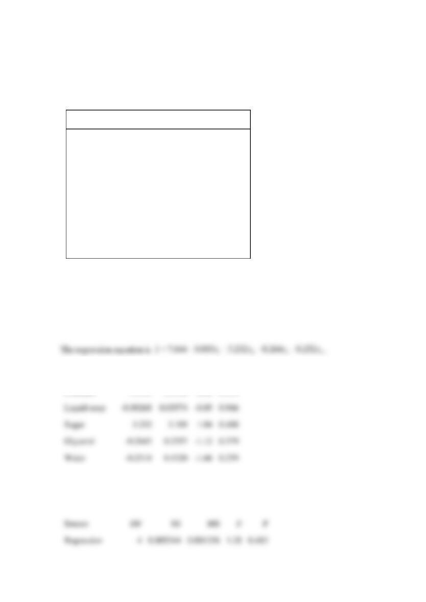
SOLUTION
Predictor
Coef
SE Coef
T
P
Constant
7.6443
0.9530
8.02
0.015
Liquid soap
-0.00268
0.05574
-0.05
0.966
Sugar
1.04
0.408
Glycerol
-0.2643
0.2357
-1.12
0.379
Water
-0.2518
0.1520
-1.66
0.239
Analysis of Variance
Source
P

Reserve Supplemental Exercises Chapter 12 Problem 4
A researcher at a Soap-Bubbles company wants to model the relationship between the quality of
solution for inflating bubbles
( )
y
and the amounts of its four main components: liquid soap
( )
1
x
, sugar
( )
2
x
, glycerol
( )
3
x
and water
( )
4
x
.
The regressors were measured in specific units. The data are shown in the following table.
Liquid soap
Sugar
Glycerol
Water
Solution
4.319
0.226
1.70
3.20
7.128
4.703
0.217
1.34
3.60
7.052
5.172
0.223
1.37
3.55
7.113
4.910
0.219
1.68
3.20
7.098
5.098
0.231
1.56
3.30
7.139
4.841
0.229
1.74
3.10
7.102
4.899
0.227
1.49
3.65
7.048
What is the value of
2
R
for the multiple linear regression model to these data?
SOLUTION
2
6