Applied Statistics and Probability for Engineers, 7th edition 2017
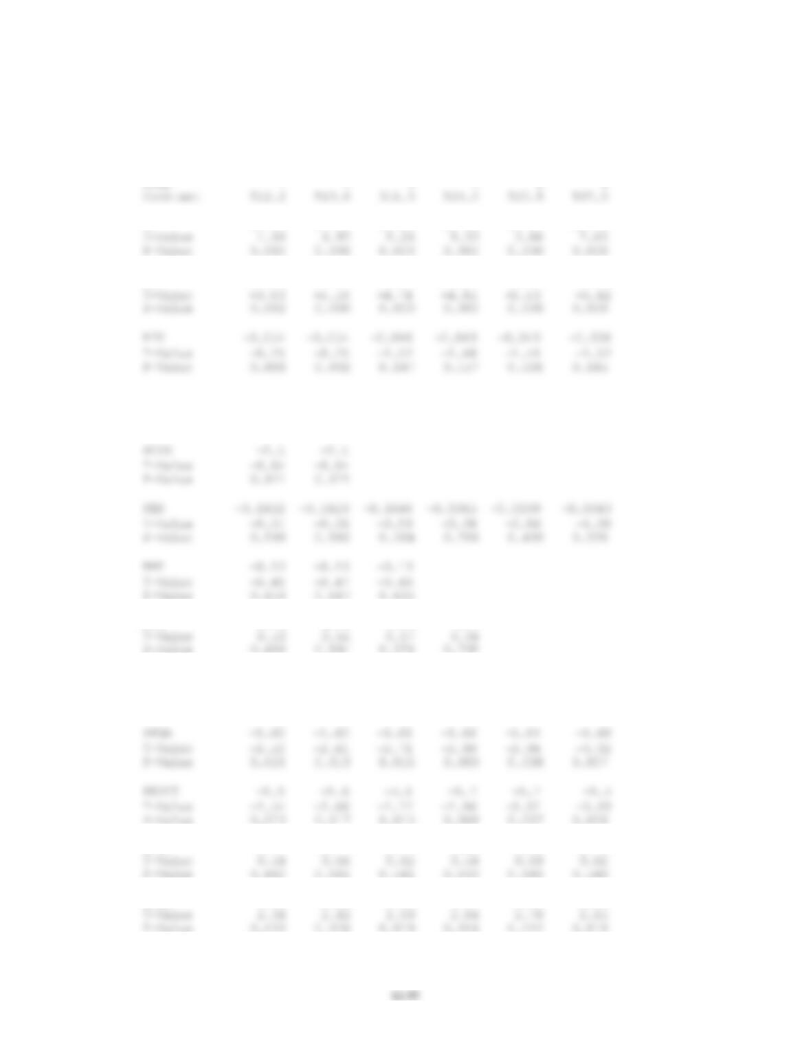
(d) Stepwise Regression: W versus GF, GA, …
Backward elimination. Alpha-to-Remove: 0.1
Response is W on 14 predictors, with N = 30
Step 1 2 3 4 5 6
GF 0.164 0.164 0.164 0.166 0.167 0.173
GA −0.183 −0.184 −0.184 −0.186 −0.190 −0.191
PPGF 0.089 0.087 0.047 0.031 0.022
T-Value 0.08 0.08 0.59 0.43 0.34
P-Value 0.938 0.937 0.565 0.671 0.739
AVG 13.1 13.1 13.2 2.7
SHT 0.29 0.29 0.29 0.31 0.31 0.30
T-Value 2.19 2.30 2.40 2.65 2.71 2.76
P-Value 0.045 0.035 0.028 0.016 0.014 0.012
SHGF 0.11 0.11 0.11 0.09 0.09 0.10
SHGA 0.61 0.61 0.61 0.57 0.54 0.53
12-56
FG 0.00
S 2.65 2.57 2.49 2.44 2.38 2.33
R-Sq 92.94 92.93 92.93 92.84 92.79 92.75
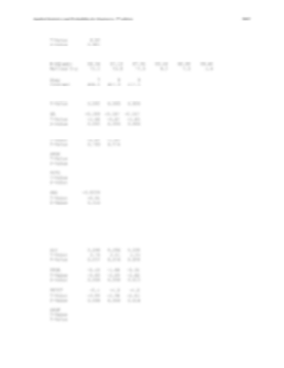
GF 0.178 0.182 0.177
T-Value 8.53 9.04 8.57
ADV −0.038 −0.038
BMI
T-Value
P-Value
AVG
T-Value
P-Value
Applied Statistics and Probability for Engineers, 7th edition 2017
12-57
SHGA 0.51 0.49 0.39
T-Value 2.83 2.74 2.23
S 2.30 2.29 2.37
R-Sq 92.60 92.29 91.34
Regression Analysis: W versus GF, GA, SHT, PPGA, PKPCT, SHGA
Predictor Coef SE Coef T P
Constant 417.5 141.3 2.95 0.007
Analysis of Variance
Source DF SS MS F P
Regression 6 1366.51 227.75 40.45 0.000
(e) There are several reasonable choices.
12.6.12 When fitting polynomial regression models, we often subtract
x
from each
x
value to produce a “centered” regressor
=−x x x
. This reduces the effects of dependencies among the model terms and often leads to more accurate estimates
of the regression coefficients. Using the data from Exercise 12.6.1, fit the model
= + + +
* * * 2
0 1 11
‘ ( ‘) .Y x x
(a) Use the results to estimate the coefficients in the uncentered model
= + + +
2
0 1 11 .Y x x
Predict y when
x = 285 °F. Suppose that you use a standardized variable
=−( ) / x
x x x s
where sx is the standard deviation of x in
constructing a polynomial regression model. Fit the model
= + + +
* * * 2
0 1 11
‘ ( ‘) .Y x x
(b) What value of y do you predict when x = 285°F?
(c) Estimate the regression coefficients in the unstandardized model
= + + +
2
0 1 11 .Y x x
Applied Statistics and Probability for Engineers, 7th edition 2017
12-58
(d) What can you say about the relationship between SSE and R2 for the standardized and unstandardized models?
(e) Suppose that
=−( ) / y
y y y s
is used in the model along with x′. Fit the model and comment on the relationship
between SSE and R2 in the standardized model and the unstandardized model.
= + +
= − −
= − − − −
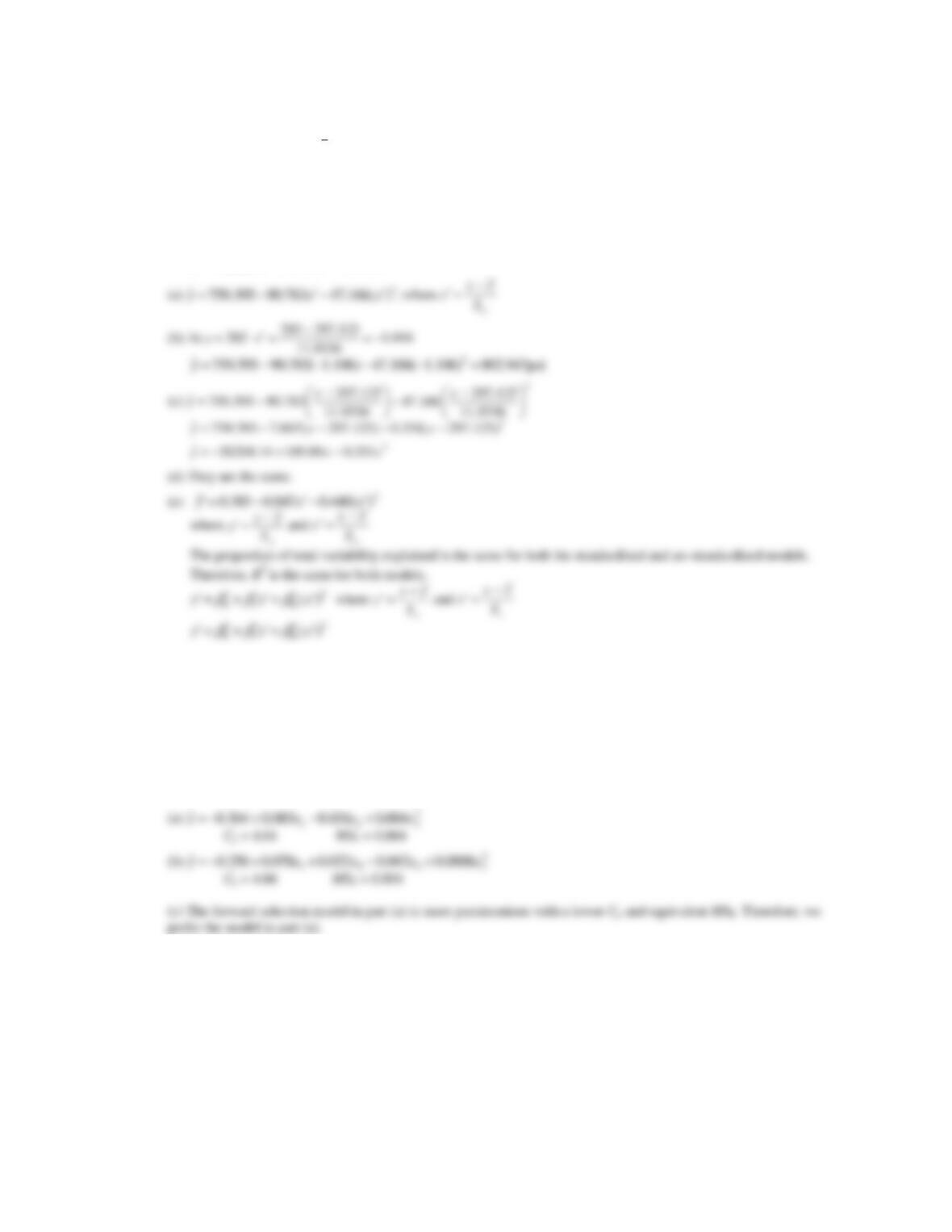
= − + −
2
0 1 11
2
2
2
ˆ()
ˆ759.395 7.607 0.331( )
ˆ759.395 7.607( 297.125) 0.331( 297.125)
ˆ26202.14 189.09 0.331
y x x
y x x
y x x
y x x
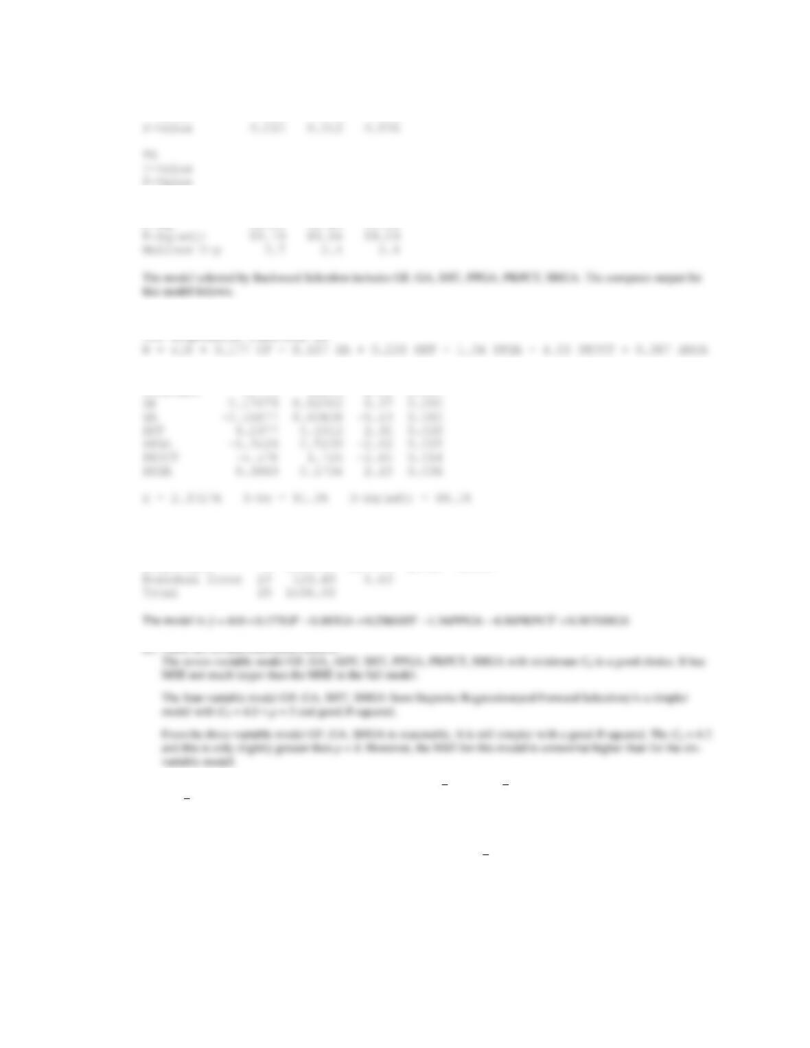
12.6.13 Consider the data in Exercise 12.6.4. Use all the terms in the full quadratic model as the candidate regressors.
(a) Use forward selection to identify a model.
(b) Use backward elimination to identify a model.
(c) Compare the two models obtained in parts (a) and (b). Which model would you prefer and why?
The default settings for F-to-enter and F-to-remove, equal to 4, were used. Different settings can change the models
generated by the method.
12.6.14 We have used a sample of 30 observations to fit a regression model. The full model has nine regressors, the variance
estimate is
==
2100
ˆE
MS
, and R2 = 0.92.
(a) Calculate the F-statistic for testing significance of regression. Using
= 0.05, what would you conclude?
(b) Suppose that we fit another model using only four of the original regressors and that the error sum of squares for
this new model is 2200. Find the estimate of
2 for this new reduced model. Would you conclude that the reduced
model is superior to the old one? Why?
(c) Find the value of Cp for the reduced model in part (b). Would you conclude that the reduced model is better than the
old model?
Applied Statistics and Probability for Engineers, 7th edition 2017
12-59
n = 30, k = 9, p = 9 + 1 = 10 in full model.
(a)
==
2
ˆ100
E
MS
=
20.92R
(b) k = 4 p = 5 SSE = 2200
12.6.15 A sample of 25 observations is used to fit a regression model in seven variables. The estimate of
2 for this full model
is MSE = 10.
(a) A forward selection algorithm has put three of the original seven regressors in the model. The error sum of squares
for the three-variable model is SSE = 300. Based on Cp, would you conclude that the three-variable model has any
remaining bias?
(b) After looking at the forward selection model in part (a), suppose you could add one more regressor to the model.
This regressor will reduce the error sum of squares to 275. Will the addition of this variable improve the model?
Why?
n = 25 k = 7 p = 8 MSE(full) = 10
(a) p = 4 SSE = 300
Applied Statistics and Probability for Engineers, 7th edition 2017
12-60
Supplemental Exercises
12.S8 Consider the following computer output.
The regression equation is
Y = 517 + 11.5 x1 − 8.14 x2 + 10.9 3
Predictor
Coef
SE Coef
T
P
Constant
517.46
11.76
?
?
x1
11.4720
?
36.50
?
x2
−8.1378
0.1969
?
?
x3
10.8565
0.6652
?
?
S = 10.2560
R-Sq = ?
R-Sq (adj) = ?
Analysis of Variance
Source
DF
SS
MS
F
P
Regression
?
347300
115767
?
?
Residual error
16
?
105
Total
19
348983
(a) Fill in the missing values. Use bounds for the P-values.
(b) Is the overall model significant at
= 0.05? Is it significant at
= 0.01?
(c) Discuss the contribution of the individual regressors to the model.
(a) The missing quantities are as follows:
== =
Constant
Coef 517.46 44.0017
Coef 11.76
TSE
Applied Statistics and Probability for Engineers, 7th edition 2017
12-61
12.S9 Consider the inverter data in Exercise 12.S10. Delete observation 2 from the original data. Define new variables as
follows: y* = lny,
=
*
11
1/xx
,
=
*
22
xx
,
=
*
33
1/xx
and
=
*
44
xx
.
(a) Fit a regression model using these transformed regressors (do not use x5 or x6).
(b) Test the model for significance of regression using
= 0.05. Use the t-test to investigate the contribution of each
variable to the model (
= 0.05). What are your conclusions?
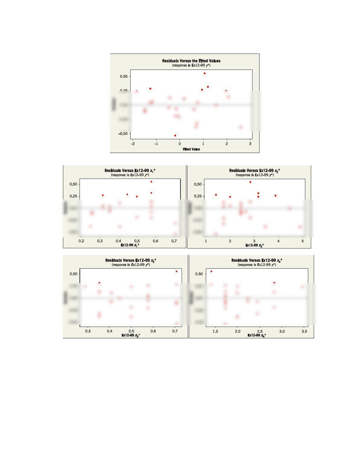
(c) Plot the residuals versus
ˆ*y
and versus each of the transformed regressors. Comment on the plots.
Note that data in row 2 are deleted to follow the instructions in the exercise.
(a)
The regression equation is
Analysis of Variance
(b) H0:
1 =
2 =
3 =
4 = 0
Applied Statistics and Probability for Engineers, 7th edition 2017
12-62
(c) The residual plots are more satisfactory than the plots in the following exercise.
12.S10 Transient points of an electronic inverter are influenced by many factors. Shown below is the data on the transient point
(y, in volts) of PMOS-NMOS inverters and five candidate regressors: x1 = width of the NMOS device, x2 = length of
the NMOS device, x3 = width of the PMOS device, x4 = length of the PMOS device, and
x5 = temperature (°C).
(a) Fit a multiple linear regression model that uses all regressors to these data. Test for significance of regression using
= 0.01. Find the P-value for this test and use it to draw your conclusions.
(b) Test the contribution of each variable to the model using the t-test with
= 0.05. What are your conclusions?
(c) Delete x5 from the model. Test the new model for significance of regression. Also test the relative contribution of
each regressor to the new model with the t-test. Using
= 0.05, what are your conclusions?

Applied Statistics and Probability for Engineers, 7th edition 2017
(d) Notice that the MSE for the model in part (c) is smaller than the MSE for the full model in part (a). Explain why this
has occurred.
(e) Calculate the studentized residuals. Do any of these seem unusually large?
(f) Suppose that you learn that the second observation was recorded incorrectly. Delete this observation and refit the
model using x1, x2, x3, and x4 as the regressors. Notice that the R2 for this model is considerably higher than the R2 for
either of the models fitted previously. Explain why the R2 for this model has increased.
(g) Test the model from part (f) for significance of regression using
= 0.05. Also investigate the contribution of each
regressor to the model using the t-test with
= 0.05. What conclusions can you draw?
Observation
Number
x1
x2
x3
x4
x5
y
1
3
3
3
3
0
0.787
2
8
30
8
8
0
0.293
3
3
6
6
6
0
1.710
4
4
4
4
12
0
0.203
5
8
7
6
5
0
0.806
6
10
20
5
5
0
4.713
7
8
6
3
3
25
0.607
8
6
24
4
4
25
9.107
9
4
10
12
4
25
9.210
10
16
12
8
4
25
1.365
11
3
10
8
8
25
4.554
12
8
3
3
3
25
0.293
13
3
6
3
3
50
2.252
14
3
8
8
3
50
9.167
15
4
8
4
8
50
0.694
16
5
2
2
2
50
0.379
17
2
2
2
3
50
0.485
18
10
15
3
3
50
3.345
19
15
6
2
3
50
0.208
20
15
6
2
3
75
0.201
21
10
4
3
3
75
0.329
22
3
8
2
2
75
4.966
23
6
6
6
4
75
1.362
24
2
3
8
6
75
1.515
25
3
3
8
8
75
0.751
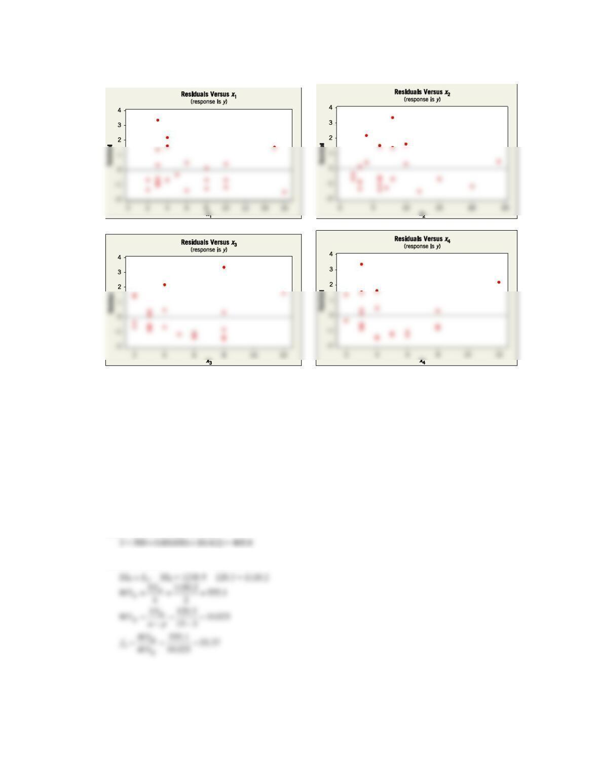
(h) Plot the residuals from the model in part (f) versus
ˆ
y
and versus each of the regressors x1, x2, x3, and x4. Comment
on the plots.
(a)
= − + + − +
ˆ2.86 0.291 0.2206 0.454 0.594 0.005y x x x x x
12-64
(b)
= 0.05 t0.025,19 = 2.093
H0:
1 = 0 H0:
2 = 0 H0:
3 = 0 H0:
4 = 0 H0:
5 = 0
H1:
1 ≠ 0 H1:
2 ≠ 0 H1:
3 ≠ 0 H1:
4 ≠ 0 H1:
5 ≠ 0
(c)
= − + + −
1 2 3 4
ˆ3.148 0.290 0.19919 0.455 0.609y x x x x
H0:
1 =
2 =
3 =
4 = 0
(e) Observation 2 is unusually large. Studentized residuals follow:
−0.80199 −4.99898 −0.39958 2.22883 −0.52268 0.62842 −0.45288 2.21003 1.37196
(f) R2 for model in part (a): 0.558.
(g) H0:
1 =
2 =
3 =
4 = 0
H1:
j ≠ 0
= 0.05
Applied Statistics and Probability for Engineers, 7th edition 2017
12-65
(h) There is some indication of curvature.
12.S11 A multiple regression model was used to relate y = viscosity of a chemical product to x1 = temperature and
x2 = reaction time. The data set consisted of n = 15 observations.
(a) The estimated regression coefficients were
=
0
ˆ 300.00
,
=
1
ˆ0.85
, and
=
21 0
ˆ0.4
. Calculate an estimate of mean
viscosity when x1 = 100°F and x2 = 2 hours.
(b) The sums of squares were SST = 1230.50 and SSE = 120.30. Test for significance of regression using
= 0.05. What
conclusion can you draw?
(c) What proportion of total variability in viscosity is accounted for by the variables in this model?
(d) Suppose that another regressor, x3 = stirring rate, is added to the model. The new value of the error sum of squares
is SSE = 117.20. Has adding the new variable resulted in a smaller value of MSE? Discuss the significance of this result.
(e) Calculate an F-statistic to assess the contribution of x3 to the model. Using
= 0.05, what conclusions do you
reach?
(a)
= + +
12
ˆ300.0 0.85 10.4y x x
(b) Syy = 1230.5 SSE = 120.3
Applied Statistics and Probability for Engineers, 7th edition 2017
12-66
H0:
1 =
2 = 0
12.S12 Consider the electronic inverter data in Exercises 12.S9 and 12.S10. Define the response and regressors variables
as in Exercise 12.S9, and delete the second observation in the sample.
(a) Use all possible regressions to find the equation that minimizes Cp.
(b) Use all possible regressions to find the equation that minimizes MSE.
(c) Use stepwise regression to select a subset regression model.
(d) Compare the models you have obtained.
(a)
= + − − −
* * * *
1 2 3 4
ˆ4.87 6.12 6.53 3.56 1.44y x x x x
12.S13 An article in the Journal of the American Ceramics Society (1992, Vol. 75, pp. 112–116) described a process for
immobilizing chemical or nuclear wastes in soil by dissolving the contaminated soil into a glass block. The authors mix
CaO and Na2O with soil and model viscosity and electrical conductivity. The electrical conductivity model involves six
regressors, and the sample consists of n = 14 observations.
(a) For the six-regressor model, suppose that SST = 0.50 and R2 = 0.94. Find SSE and SSR, and use this information to
test for significance of regression with α = 0.05. What are your conclusions?
Applied Statistics and Probability for Engineers, 7th edition 2017
12-67
(b) Suppose that one of the original regressors is deleted from the model, resulting in R2 = 0.92. What can
you conclude about the contribution of the variable that was removed? Answer this question by calculating an
F-statistic.
(c) Does deletion of the regressor variable in part (b) result in a smaller value of MSE for the five-variable model, in
comparison to the original six-variable model? Comment on the significance of your answer.
(a)
=
2R
SS
RS
12.S14 Exercise 12.1.5 introduced the hospital patient satisfaction survey data. One of the variables in that data set is a
categorical variable indicating whether the patient is a medical patient or a surgical patient. Fit a model including this
indicatorvariable to the data using all three of the other regressors. Is there any evidence that the service the patient is
on (medical versus surgical) has an impact on the reported satisfaction?
The computer output is shown below. The P-value of the Surg-Med indicator variable (third variable) is greater than
= 0.05, so we fail to reject the H0 and conclude that Surg-Med indicator variable does not contribute significantly to the
model. Thus, the surgical and medical service does not impact the reported satisfaction.
Applied Statistics and Probability for Engineers, 7th edition 2017
Regression Analysis: Satisfaction versus Age, Severity, …
The regression equation is
Satisfaction = 144 – 1.12 Age – 0.586 Severity + 0.41 Surg-Med + 1.31 Anxiety
Predictor Coef SE Coef T P
Constant 143.867 6.044 23.80 0.000
Age -1.1172 0.1383 -8.08 0.000
Analysis of Variance
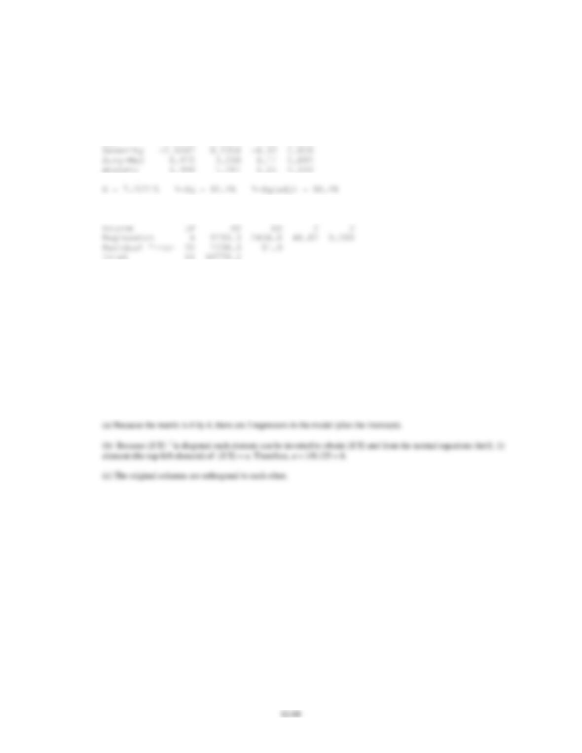
12.S15 Consider the following inverse model matrix.
−
=
1
0.125 0 0 0
0 0.125 0 0
() 0 0 0.125 0
0 0 0 0.125
XX
(a) How many regressors are in this model?
(b) What was the sample size?
(c) Notice the special diagonal structure of the matrix. What does that tell you about the columns in the
original X matrix?