
12-41
Applied Statistics and Probability for Engineers, 7th edition 2017
12-42
Sections 12.6
12.6.1 An article entitled “A Method for Improving the Accuracy of Polynomial Regression Analysis” in the Journal of
Quality Technology (1971, pp. 149–155) reported the following data on y = ultimate shear strength of a rubber
compound(psi) and x = cure temperature (°F).
y
770
800
840
x
280
284
292
y
735
640
590
x
298
305
308
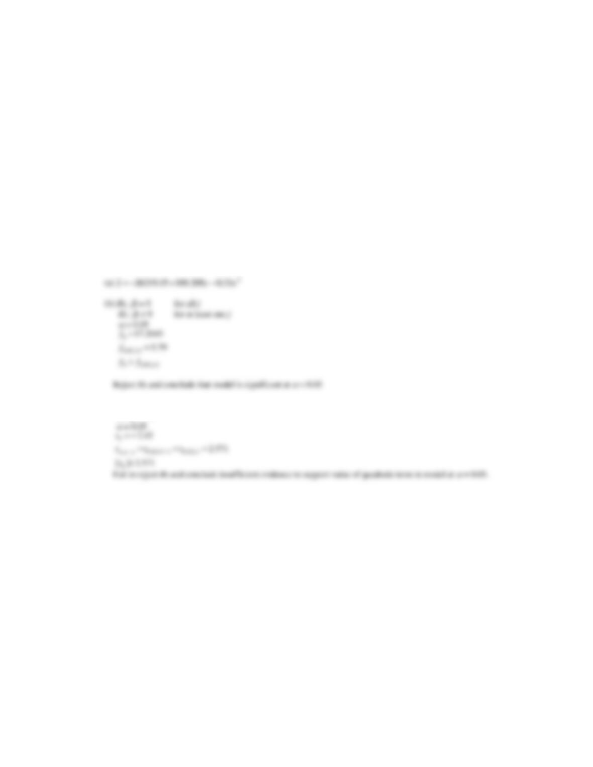
(a) Fit a second-order polynomial to these data.
(b) Test for significance of regression using
= 0.05.
(c) Test the hypothesis that
11 = 0 using
= 0.05.
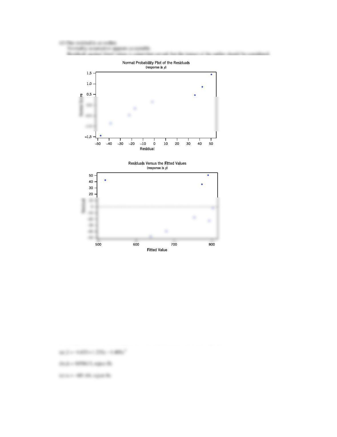
(d) Compute the residuals from part (a) and use them to evaluate model adequacy.
(c) H0:
11 = 0
H1:
11 ≠ 0
Applied Statistics and Probability for Engineers, 7th edition 2017
12-43
12.6.2 Consider the following data, which result from an experiment to determine the effect of x = test time in hours at a
particular temperature on y = change in oil viscosity:
(a) Fit a second-order polynomial to the data.
y
−1.42
−1.39
−1.55
−1.89
−2.43
x
.25
.50
.75
1.00
1.25
y
−3.15
−4.05
−5.15
−6.43
−7.89
x
1.50
1.75
2.00
2.25
2.50
(b) Test for significance of regression using
= 0.05.
(c) Test the hypothesis that
11 = 0 using
= 0.05.
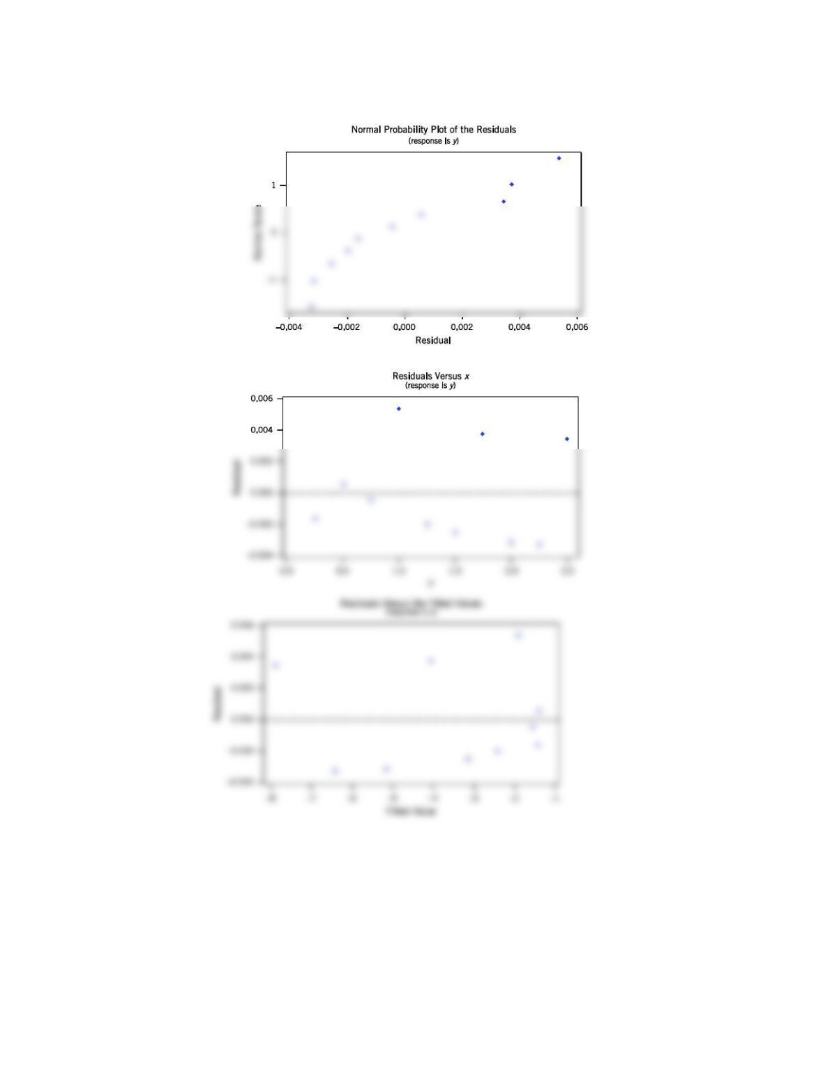
(d) Compute the residuals from part (a) and use them to evaluate model adequacy.
Applied Statistics and Probability for Engineers, 7th edition 2017
12-44
(d) Model is acceptable. Observation number 10 has large leverage.
Applied Statistics and Probability for Engineers, 7th edition 2017
12-45
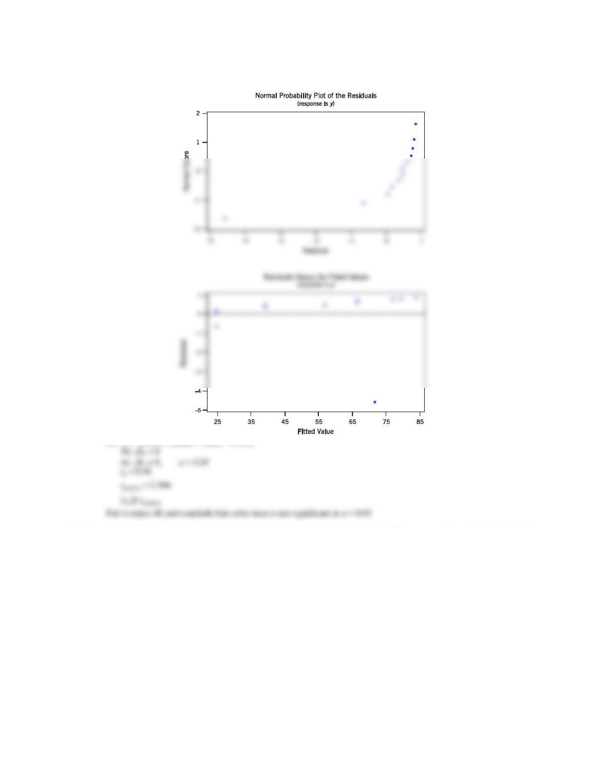
12.6.3 The following data were collected during an experiment to determine the change in thrust efficiency (y, in percent) as
the divergence angle of a rocket nozzle (x) changes:
y
24.60
24.71
23.90
39.50
39.60
57.12
x
4.0
4.0
4.0
5.0
5.0
6.0
y
67.11
67.24
67.15
77.87
80.11
84.67
x
6.5
6.5
6.75
7.0
7.1
7.3
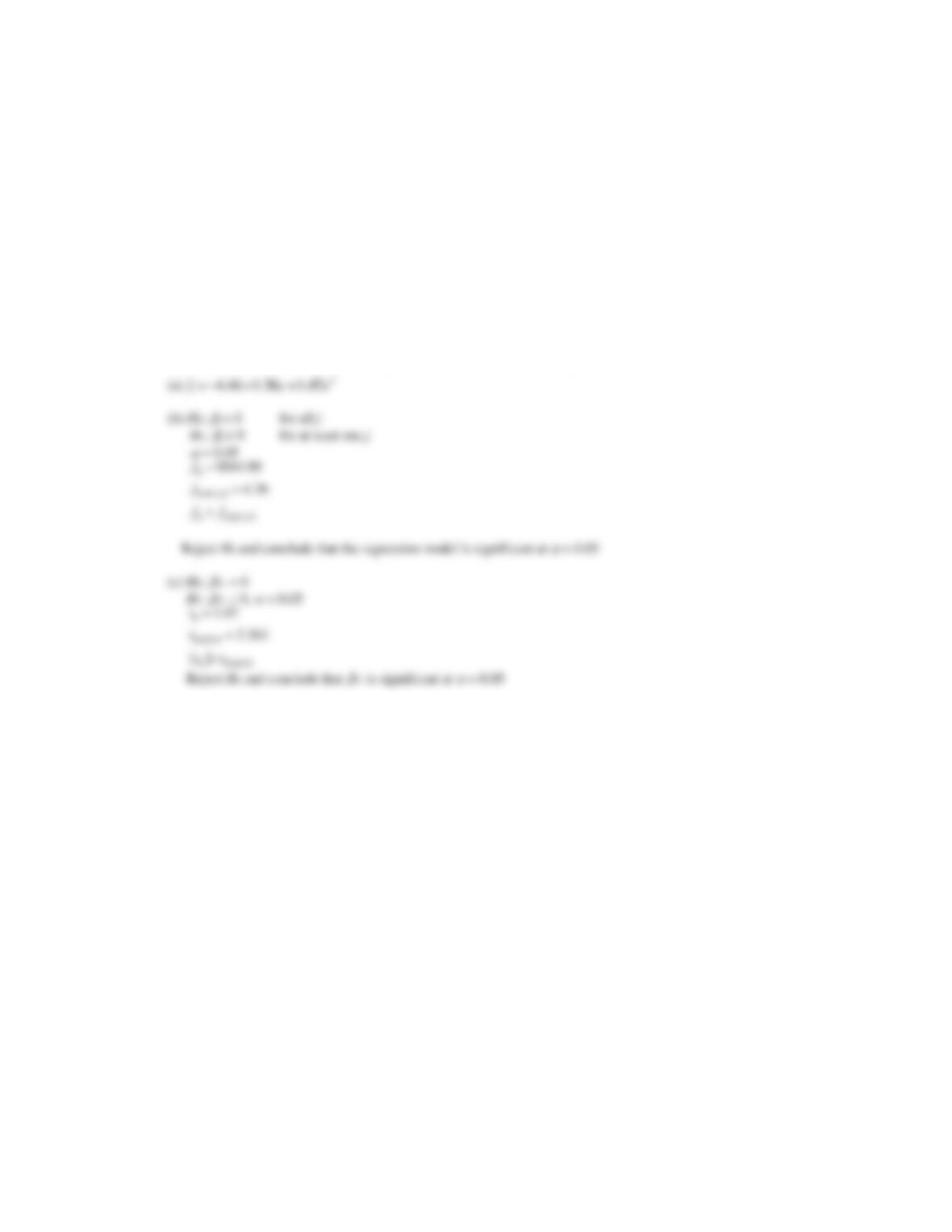
(a) Fit a second-order model to the data.
(b) Test for significance of regression and lack of fit using
= 0.05.
(c) Test the hypothesis that
11 = 0, using
= 0.05.
(d) Plot the residuals and comment on model adequacy.
(e) Fit a cubic model, and test for the significance of the cubic term using
= 0.05.
Applied Statistics and Probability for Engineers, 7th edition 2017
12-46
(d) Observation 9 is an extreme outlier. Data does not appear normal.
(e)
= − + − +
23
ˆ87.36 48.01 7.04 0.51y x x x
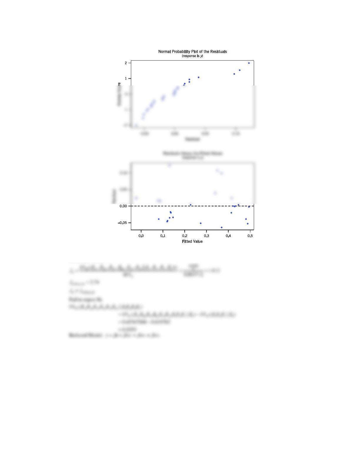
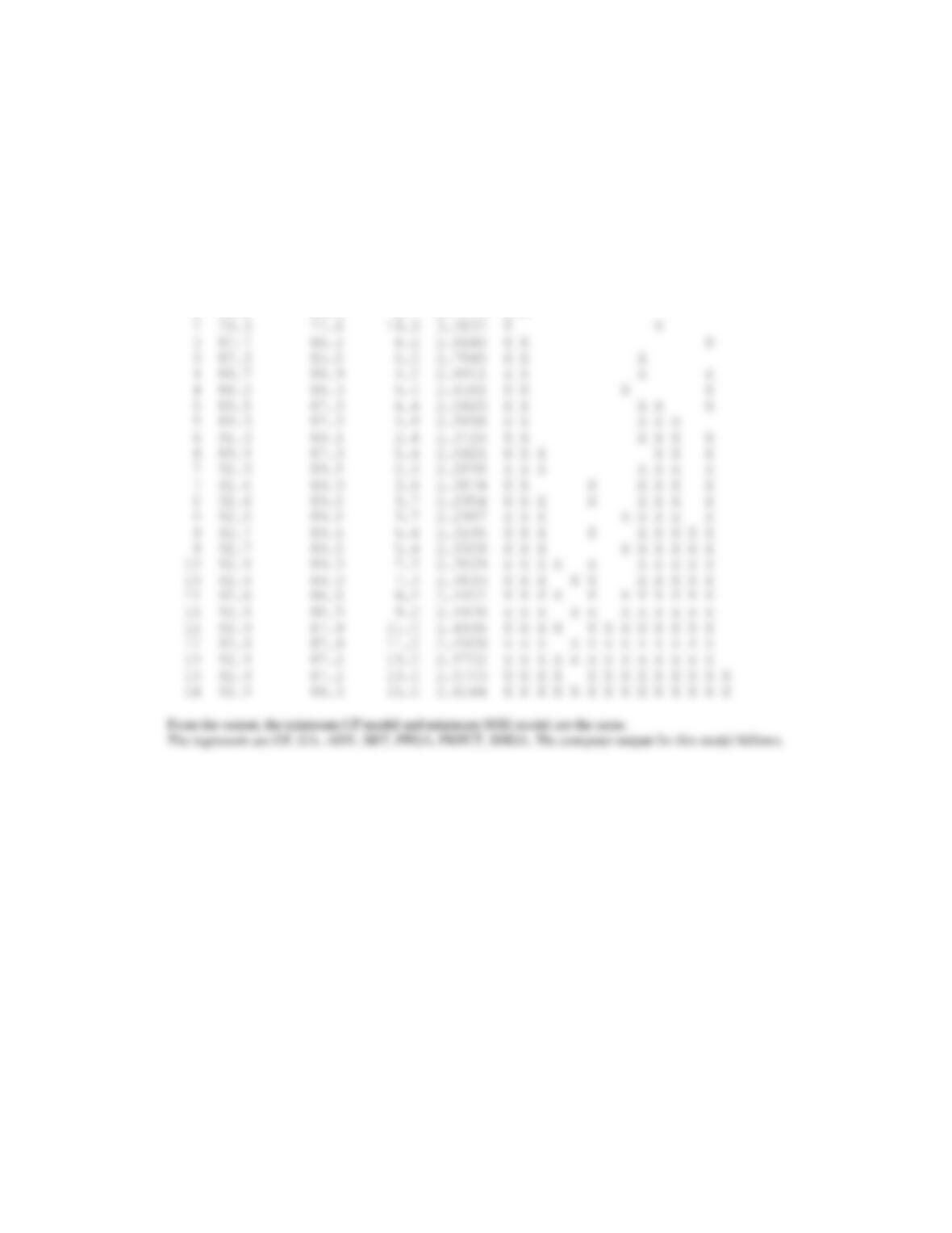
12.6.4 An article in the Journal of Pharmaceuticals Sciences (1991, Vol. 80, pp. 971–977) presents data on the observed mole
fraction solubility of a solute at a constant temperature and the dispersion, dipolar, and hydrogen-bonding Hansen
partial solubility parameters. The data are as shown in the Table E12-13, where y is the negative logarithm of the mole
fraction solubility, x1 is the dispersion partial solubility, x2 is the dipolar partial solubility, and x3 is the hydrogen-
bonding partial solubility.
(a) Fit the model
= + + + + + + + + + +
2 2 2
0 1 1 2 2 3 3 12 1 2 13 1 3 23 2 3 11 1 22 2 33 3 .Y x x x x x x x x x x x x
(b) Test for significance of regression using
= 0.05.
(c) Plot the residuals and comment on model adequacy.
Applied Statistics and Probability for Engineers, 7th edition 2017
12-47
(d) Use the extra sum of squares method to test the contribution of the second-order terms using
= 0.05.
Observation
Number
y
1
x
x2
x3
1
0.22200
7.3
0.0
0.0
2
0.39500
8.7
0.0
0.3
3
0.42200
8.8
0.7
1.0
4
0.43700
8.1
4.0
0.2
5
0.42800
9.0
0.5
1.0
6
0.46700
8.7
1.5
2.8
7
0.44400
9.3
2.1
1.0
8
0.37800
7.6
5.1
3.4
9
0.49400
10.0
0.0
0.3
10
0.45600
8.4
3.7
4.1
11
0.45200
9.3
3.6
2.0
12
0.11200
7.7
2.8
7.1
13
0.43200
9.8
4.2
2.0
14
0.10100
7.3
2.5
6.8
15
0.23200
8.5
2.0
6.6
16
0.30600
9.5
2.5
5.0
17
0.09230
7.4
2.8
7.8
18
0.11600
7.8
2.8
7.7
19
0.07640
7.7
3.0
8.0
20
0.43900
10.3
1.7
4.2
21
0.09440
7.8
3.3
8.5
22
0.11700
7.1
3.9
6.6
23
0.07260
7.7
4.3
9.5
24
0.04120
7.4
6.0
10.9
25
0.25100
7.3
2.0
5.2
26
0.00002
7.6
7.8
20.7
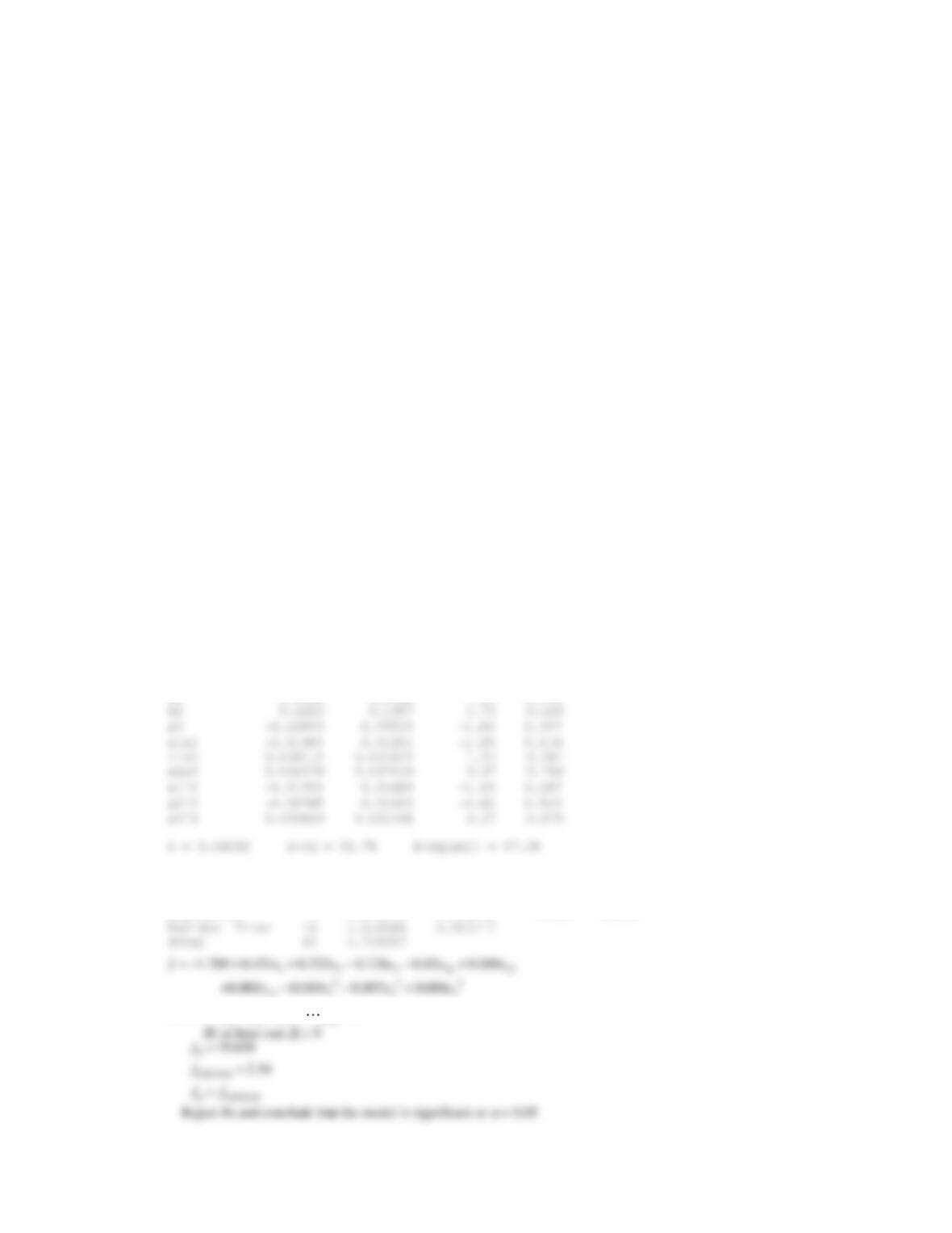
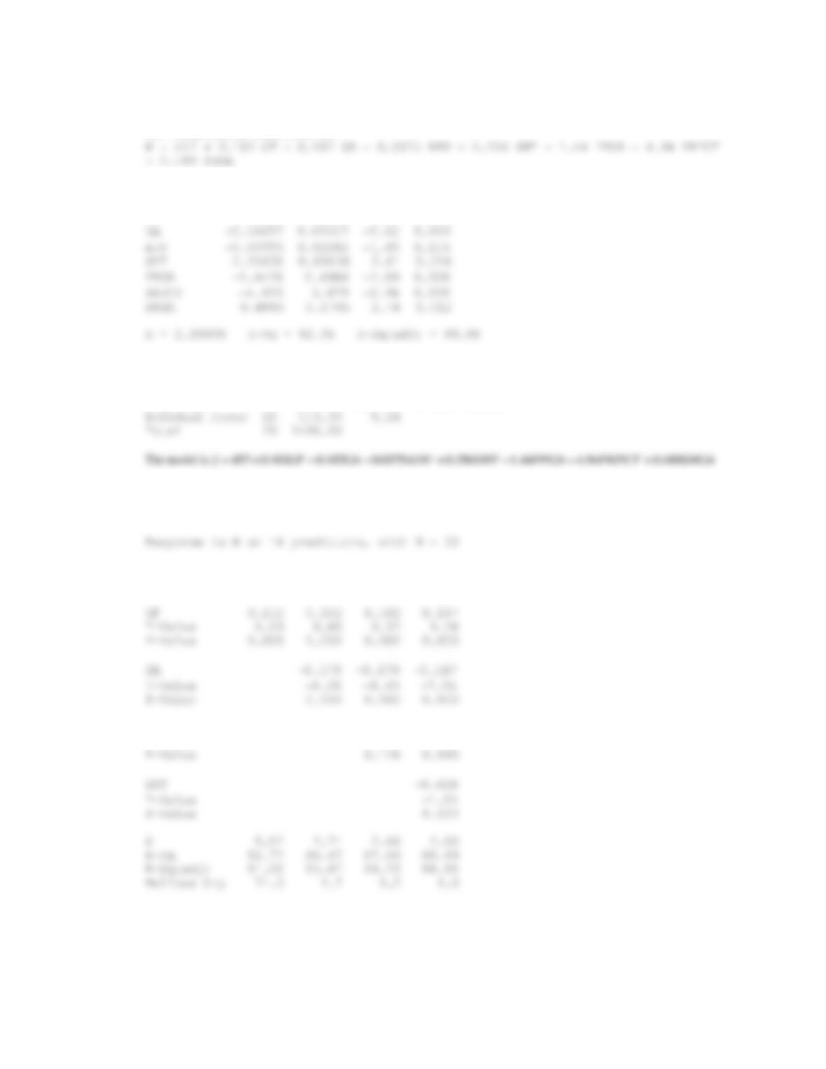
(a) Predictor Coef SE Coef T P
Constant −1.769 1.287 −1.37 0.188
xl 0.4208 0.2942 1.43 0.172
Analysis of Variance
Source DF SS MS F P
Regression 9 0.655671 0.072852 19.63 0.000
(b) H0 all
= = = =
1 2 3 23 0
Applied Statistics and Probability for Engineers, 7th edition 2017
12-48
(c) Assumptions appear to be reasonable.
(d) H0:
11 =
22 =
33 =
12 =
13 =
23 = 0
H1 at least one
≠ 0
12.6.5 Consider the electric power data in Exercise 12.1.6. Build regression models for the data using the following
techniques:
(a) All possible regressions. Find the minimum Cp and minimum MSE equations.
(b) Stepwise regression.
(c) Forward selection.
(d) Backward elimination.
(e) Comment on the models obtained. Which model would you prefer?
The default settings for F-to-enter and F-to-remove, equal to 4, in the computer software were used. Different settings
can change the models generated by the method.
Applied Statistics and Probability for Engineers, 7th edition 2017
12-49
(a)
The min MSE model is x1, x2, x 3
12.6.6 Consider the X-ray inspection data in Exercise 12.1.7. Use rads as the response. Build regression models for the data
using the following techniques:
(a) All possible regressions.
(b) Stepwise regression.
(c) Forward selection.
(d) Backward elimination.
(e) Comment on the models obtained. Which model would you prefer? Why?
12.6.7 Consider the wire bond pull strength data in Exercise 12.1.8. Build regression models for the data using the following
methods:
(a) All possible regressions. Find the minimum Cp and minimum MSE equations.
(b) Stepwise regression.
(c) Forward selection.
(d) Backward elimination.
(e) Comment on the models obtained. Which model would you prefer?
The default settings for F-to-enter and F-to-remove for Minitab were used. Different settings can change the models
generated by the method.
Applied Statistics and Probability for Engineers, 7th edition 2017
12-50
(a)
12.6.8 Consider the regression model fit to the coal and limestone mixture data in Exercise 12.1.9. Use density as the
response. Build regression models for the data using the following techniques:
(a) All possible regressions.
(b) Stepwise regression.
(c) Forward selection.
(d) Backward elimination.
(e) Comment on the models obtained. Which model would you prefer? Why?
(a) The min Cp model is x1
12.6.9 Consider the nisin extraction data in Exercise 12.1.10. Build regression models for the data using the following
techniques:
(a) All possible regressions.
(b) Stepwise regression.
(c) Forward selection.
(d) Backward elimination.
(e) Comment on the models obtained. Which model would you prefer? Why?
Applied Statistics and Probability for Engineers, 7th edition 2017
12-51
(a) The min Cp model is x1,x2
12.6.10 Consider the gray range modulation data in Exercise 12.1.11. Use the useful range as the response. Build regression
models for the data using the following techniques:
(a) All possible regressions.
(b) Stepwise regression.
(c) Forward selection.
(d) Backward elimination.
(f) Comment on the models obtained. Which model would you prefer? Why?
(a) The min Cp model is x2
12.6.11 Consider the NHL data in Exercise 12.1.12. Build regression models for these data with regressors GF through FG
using the following methods:
(a) All possible regressions. Find the minimum Cp and minimum MSE equations.
(b) Stepwise regression.
(c) Forward selection.
(d) Backward elimination.
(e) Which model would you prefer?
The default settings for F-to-enter and F-to-remove for Minitab were used. Different settings can change the models
generated by the method.
Applied Statistics and Probability for Engineers, 7th edition 2017
12-52
(a)
Best Subsets Regression: W versus GF, GA, …
Response is W
P
P P P K S S
A P C P B A S P P H H
Mallows G G D G T E M V H G C G G F
Vars R-Sq R-Sq(adj) C-p S F A V F G N I G T A T F A G
1 52.8 51.1 74.3 5.0233 X
1 49.3 47.5 81.6 5.2043 X
2 86.5 85.5 4.7 2.7378 X X
Applied Statistics and Probability for Engineers, 7th edition 2017
12-53
Regression Analysis: W versus GF, GA, ADV, SHT, PPGA, PKPCT, SHGA
The regression equation is
Predictor Coef SE Coef T P
Constant 457.3 138.5 3.30 0.003
GF 0.18233 0.02018 9.04 0.000
Analysis of Variance
Source DF SS MS F P
Regression 7 1380.70 197.24 37.63 0.000
(b) Stepwise Regression: W versus GF, GA, …
Alpha-to-Enter: 0.15 Alpha-to-Remove: 0.15
Step 1 2 3 4
Constant −8.574 40.271 38.311 43.164
SHGA 0.27 0.29
T-Value 1.58 1.76
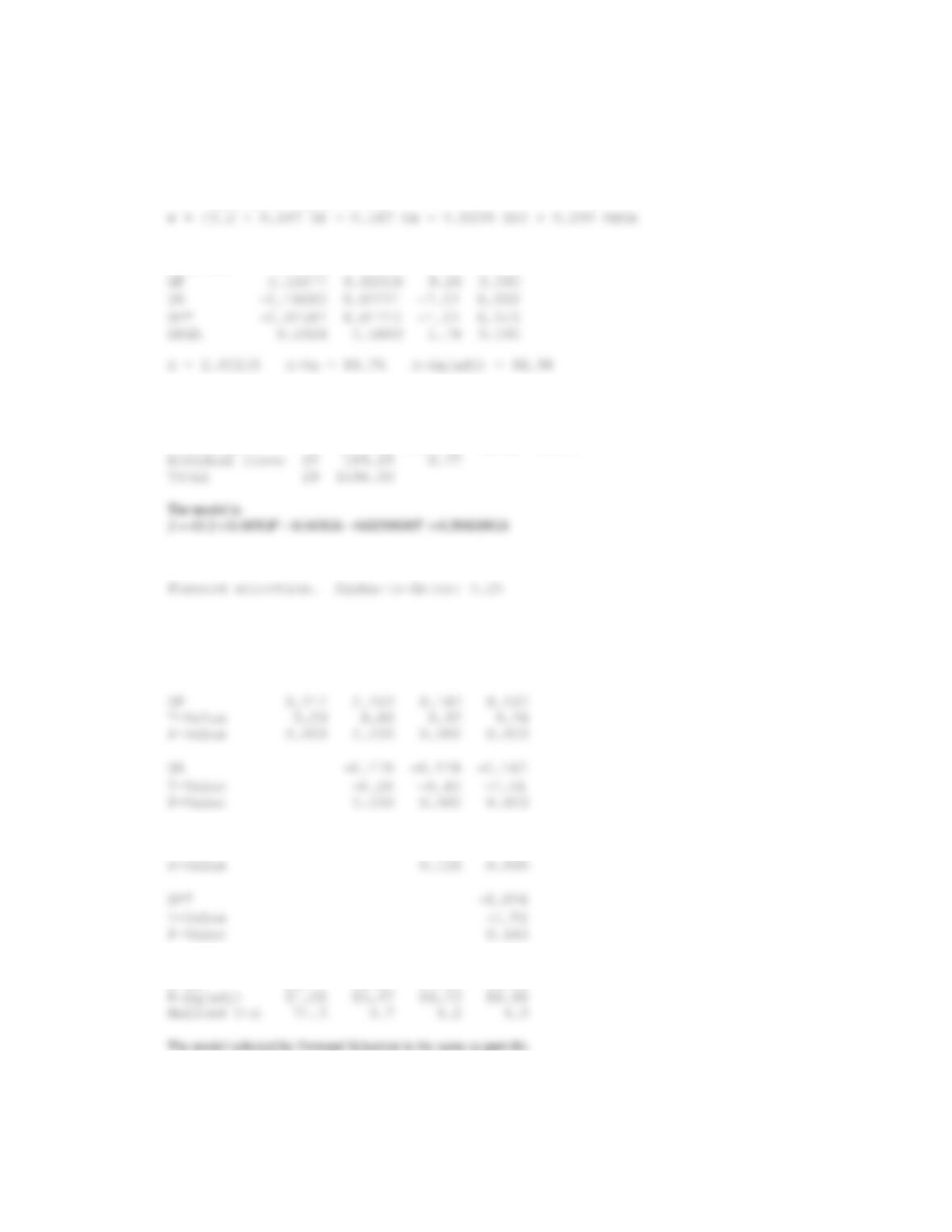
Applied Statistics and Probability for Engineers, 7th edition 2017
12-54
The selected model from Stepwise Regression has four regressorsGF, GA, SHT, SHGA. The computer output for this
model follows.
Regression Analysis: W versus GF, GA, SHT, SHGA
The regression equation is
PredictorCoef SE Coef T P
Constant 43.164 8.066 5.35 0.000
Analysis of Variance
Source DF SS MS F P
Regression 4 1326.85 331.71 49.03 0.000
(c) Stepwise Regression: W versus GF, GA, …
Response is W on 14 predictors, with N = 30
Step 1 2 3 4
Constant −8.574 40.271 38.311 43.164
SHGA 0.27 0.29
T-Value 1.58 1.76
S 5.02 2.74 2.66 2.60
R-Sq 52.77 86.47 87.66 88.69