
CHAPTER 12 RESERVE PROBLEMS
The following problems have been reserved for your use in assignments and testing and do not
appear in student versions of the text.
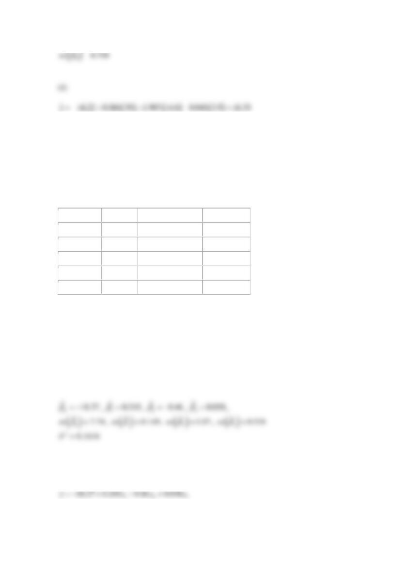
Reserve Problems Chapter 12 Section 1 Problem 1
During a research, the amount of Internet users was measured. Each time three random groups of
10 thousand people of the average age of 20, 40, and 60 were considered. The data are as follows
(
1
x
– the number of years since the beginning of the research,
2
x
– age, y – number of users):
y
1700
1450
220
3300
2800
570
4750
4410
1110
6490
5930
1520
1
x
1
1
1
3
3
3
5
5
5
7
7
7
2
x
20
40
60
20
40
60
20
40
60
20
40
60
(a) Fit a multiple linear regression model using
1
x
and
2
x
as the regressors.
(b) Estimate
2
.
(c) Find the standard errors of the regression coefficients.
(d) Use the model to predict the number of users in random group of 40 years after 4 years of
research.
SOLUTION
Using Minitab following values are obtained:
(b)
(c)
(d)

Reserve Problems Chapter 12 Section 1 Problem 2
The diameter of an oak trunk (y) depends on its age (
1
x
), height (
2
x
) and diameter of its crown (
3
x
). The results of measurements are as follows:
Trunk diameter, cm
Age, years
Height, m
Crown diameter, m
7.1
21
9.8
1.1
8.5
37
10.2
3.1
10.6
35
12.7
1.6
13.6
36
13.9
2.1
16.0
42
15.2
4.6
18.7
46
15.3
3.7
19.8
44
16.8
5.6
20.5
41
16.5
6.3
24.3
45
16.9
4.0
(a) Fit a multiple linear regression model using age, height and crown diameter as the regressors.
(b) Estimate
2
.
(c) Find the standard errors of the regression coefficients.
(d) Estimate the trunk diameter for a 39-year oak which has the height of 14.6 meters and the
crown diameter of 3.9 meters.
SOLUTION
Using Minitab following values are obtained:
014.22
ˆ
=−
,
10.066
ˆ
=
,
21.907
ˆ
=
,
3
ˆ0.04
=
,
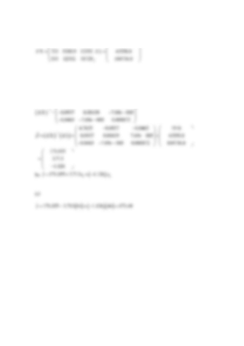
Reserve Problems Chapter 12 Section 1 Problem 3
A movie theater chain has calculated the total rating y for five films. Following parameters were
used in the estimation – audience
1
x
(number of viewers in thousands of people), coefficient
based on length of film
2
x
, critics’‘ rating
3
x
, and coefficient based on personal opinion of movie
theater chain owners which will be considered as random error. The results are shown in the
table:
Total rating
Audience
Length coefficient
Critics rating
11.55
136.8
8.1
7.9
7.71
116.1
6.2
5.9
13.27
144.2
9.3
8.1
11.79
134.6
7.3
9.4
8.46
121.8
7.0
6.8
(a) Fit a multiple linear regression model to these data.
(b) Estimate
2
.
(c) Find the standard errors of the regression coefficients.
(d) Estimate the total rating for a film that has a length coefficient of 8.4, critics’‘ rating of 7.2
and was watched by 150000 viewers.
SOLUTION
Using Minitab following values are obtained:
(a)
(b)
(c)
Reserve Problems Chapter 12 Section 1 Problem 4
Consider the multiple linear regression model
0 1 1 2 2
Y x x
= + + +
. How will the regression
coefficients change in case of new regressor variables
11
59zx=+
,
22
3zx=+
?
SOLUTION
1
1 1 1
9
59 5
z
z x x −
= + =
Reserve Problems Chapter 12 Section 1 Problem 5
A study was performed to investigate the shear strength of soil (y) as it related to depth in feet
(
1
x
) and percent of moisture content (
2
x
). Ten observations were collected, and the following
summary quantities obtained:
10n=
,
1223
i
x=
,
2553
i
x=
,
1916
i
y=
,
2
15200.9
i
x=
,
2
231729
i
x=
,
12
12352
ii
xx=
,
143550.8
ii
xy=
,
2104736.8
ii
xy=
, and
2371595.6
i
y=
.
(a) Set up the least squares normal equations for the model
0 1 1 2 2
Y x x
= + + +
.
(b) Estimate the parameters in the model in part (a).
(c) What is the predicted strength when
1
x
= 14 feet and
2
x
= 44%?
SOLUTION
(a)
10 223 553 1916
(b)
( ) ( )
1
ˆX X X y
−
=
4.7625 0.0937 0.0465
−−
Reserve Problems Chapter 12 Section 1 Problem 6
A chemical engineer is investigating how the amount of conversion of a product from a raw
material (y) depends on reaction temperature (
1
x
) and the reaction time (
2
x
). He has developed
the following regression models:
1.
12
100 2 4
ˆ
y x x= + +
2.
1 2 1 2
ˆ95 1.5 3 2y x x x x= + + +
Both models have been built over the range
2
0.5 10.x
(a) What is the predicted value of conversion when
2
x
= 3?
(b) Repeat this calculation for
2
x
= 6.
(c) Find the expected change in the mean conversion for a unit change in temperature
1
x
for
model 2 when
22x=
and
28x=
.
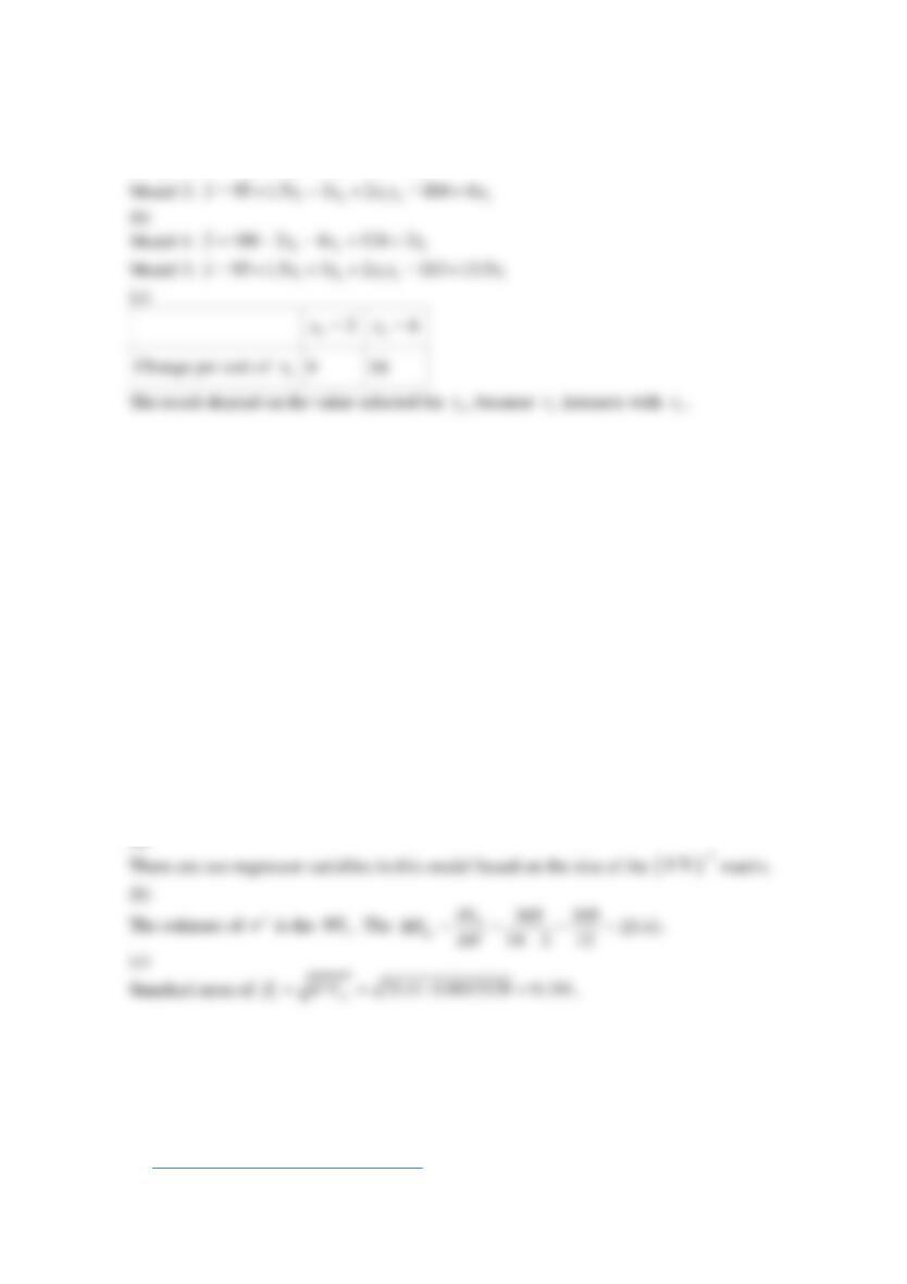
SOLUTION
(a)
Model 1:
1 2 1
100 2 4
ˆ112 2y x x x= + + = +
Reserve Problems Chapter 12 Section 1 Problem 7
You have fit a multiple linear regression model and the
( )
1
XX −
matrix is:
( )
1
0.893758 0.0282448 0.0175641
0.028245 0.0013329 0.0001547
0.017564 0.0001547 0.0009108
XX −
−−
=−
−
(a) How many regressor variables are in this model?
(b) If the error sum squares is 305 and there are 14 observations, what is the estimate of
2
?
(c) What is the standard error of the regression coefficient
1
ˆ
?
SOLUTION
(a)
Reserve Problems Chapter 12 Section 1 Problem 8
Table provides the highway gasoline mileage test results for 2005 model year vehicles from
DaimlerChrysler. The full table of data (available on the book’s Web site) contains the same data
for 2005 models from over 250 vehicles from many manufacturers (Environmental Protection AgencyWeb
site www.epa.gov/otaq/cert/mpg/testcars/database).
1 2 1
100 2 4
ˆ124 2y x x x= + + = +

Table DaimlerChrysler Fuel Economy and Emissions
mfr
carline
car/truck
cid
rhp
trns
drv
od
etw
cmp
axle
n/v
a/c
hc
co
co2
mpg
20
300C/SRT-8
C
215
253
L5
4
2
4500
9.9
3.07
30.9
Y
0.011
0.09
288
30.8
20
CARAVAN 2WD
C
201
180
L4
F
2
4500
9.3
2.49
32.3
Y
0.014
0.11
274
32.5
20
CROSSFIRE ROADSTER
C
196
168
L5
R
2
3375
10
3.27
37.1
Y
0.001
0.02
250
35.4
20
DAKOTA PICKUP 2WD
C
226
210
L4
R
2
4500
9.2
3.55
29.6
Y
0.012
0.04
316
28.1
20
DAKOTA PICKUP 4WD
C
226
210
L4
4
2
5000
9.2
3.55
29.6
Y
0.011
0.05
365
24.4
20
DURANGO 2WD
C
348
345
L5
R
2
5250
8.6
3.55
27.2
Y
0.023
0.15
367
24.1
20
GRAND CHEROKEE 2WD
C
226
210
L4
R
2
4500
9.2
3.07
30.4
Y
0.006
0.09
312
28.5
20
GRAND CHEROKEE 4WD
C
348
230
L5
4
2
5000
9
3.07
24.7
Y
0.008
0.11
369
24.2
20
LIBERTY/CHEROKEE 2WD
C
148
150
M6
R
2
4000
9.5
4.1
41
Y
0.004
0.41
270
32.8
20
LIBERTY/CHEROKEE 4WD
C
226
210
L4
4
2
4250
9.2
3.73
31.2
Y
0.003
0.04
317
28
20
NEON/SRT-4/SX 2.0
C
122
132
L4
F
2
3000
9.8
2.69
39.2
Y
0.003
0.16
214
41.3
20
PACIFICA 2WD
C
215
249
L4
F
2
4750
9.9
2.95
35.3
Y
0.022
0.01
295
30
20
PACIFICA AWD
C
215
249
L4
4
2
5000
9.9
2.95
35.3
Y
0.024
0.05
314
28.2
20
PT CRUISER
C
148
220
L4
F
2
3625
9.5
2.69
37.3
Y
0.002
0.03
260
34.1
20
RAM 1500 PICKUP 2WD
C
500
500
M6
R
2
5250
9.6
4.1
22.3
Y
0.01
0.1
474
18.7
20
RAM 1500 PICKUP 4WD
C
348
345
L5
4
2
6000
8.6
3.92
29
Y
0
0
0
20.3
20
SEBRING 4-DR
C
165
200
L4
F
2
3625
9.7
2.69
36.8
Y
0.011
0.12
252
35.1
20
STRATUS 4-DR
C
148
167
L4
F
2
3500
9.5
2.69
36.8
Y
0.002
0.06
233
37.9
20
TOWN & COUNTRY 2WD
C
148
150
L4
F
2
4250
9.4
2.69
34.9
Y
0
0.09
262
33.8

20
VIPER CONVERTIBLE
C
500
501
M6
R
2
3750
9.6
3.07
19.4
Y
0.007
0.05
342
25.9
20
WRANGLER/TJ 4WD
C
148
150
M6
4
2
3625
9.5
3.73
40.1
Y
0.004
0.43
337
26.4
mfr-mfr code
carline-car line name (test vehicle model name)
car/truck-‘C’ for passenger vehicle and ‘T’ for truck
cid-cubic inch displacement of test vehicle
rhp-rated horsepower
trns-transmission code
drv-drive system code
od-overdrive code
etw-equivalent test weight
cmp-compression ratio
axle-axle ratio
n/v-n/v ratio (engine speed versus vehicle speed at 50 mph)
a/c-indicates air conditioning simulation
hc-HC(hydrocarbon emissions) Test level composite results
co-CO(carbon monoxide emissions) Test level composite results
co2-CO2(carbon dioxide emissions) Test level composite results
mpg-mpg(fuel economy, miles per gallon)
(a) Fit a multiple linear regression model to these data to estimate gasoline mileage that uses the following regressors: cid, rhp, etw, cmp, axle, n/ν.
(b) Estimate
2
and the standard errors of the regression coefficients.
(c) Predict the gasoline mileage for the first vehicle in the table.

SOLUTION
(a)
Reserve Problems Chapter 12 Section 1 Problem 9
An engineer at a semiconductor company wants to model the relationship between the device
HFE (y) and three parameters: Emitter-RS (
1
x
), Base-RS (
2
x
), and Emitter-to-Base RS (
3
x
).
The data are shown in the Table.
Table Semiconductor Data.
x1
Emitter-RS
x2
Base-RS
x3
E-B-RS
y
HFE-1M-5V
14.62
226
7
128.4
15.63
220
3.375
52.62
14.62
217.4
6.375
113.9
15
220
6
98.01
14.5
226.5
7.625
139.9
15.25
224.1
6
102.6
16.12
220.5
3.375
48.14
15.13
223.5
6.125
109.6
15.5
217.6
5
82.68
15.13
228.5
6.625
112.6
15.5
230.2
5.75
97.52
16.12
226.5
3.75
59.06
15.13
226.6
6.125
111.8
15.63
225.6
5.375
89.09

15.38
229.7
5.875
101
14.38
234
8.875
171.9
15.5
230
4
66.8
14.25
224.3
8
157.1
14.5
240.5
10.87
208.4
14.62
223.7
7.375
133.4
(a) Fit a multiple linear regression model to the data.
(b) Estimate
2
.
(c) Predict HFE when
1 2 3
14.5, 225, and 4.5.x x x= = =
SOLUTION
(a)
Reserve Problems Chapter 12 Section 1 Problem 10
Heat treating is often used to carburize metal parts such as gears. The thickness of the carburized
layer is considered a crucial feature of the gear and contributes to the overall reliability of the
part. Because of the critical nature of this feature, two different lab tests are performed on each
furnace load. One test is run on a sample pin that accompanies each load. The other test is a
destructive test that cross-sections an actual part. This test involves running a carbon analysis on
the surface of both the gear pitch (top of the gear tooth) and the gear root (between the gear
teeth). Table shows the results of the pitch carbon analysis test for 32 parts. The regressors are furnace
temperature (TEMP), carbon concentration and duration of the carburizing cycle (SOAKPCT,
SOAKTIME), and carbon concentration and duration of the diffuse cycle (DIFFPCT,
DIFFTIME).
Table Heat Treating Test
TEMP
SOAKTIME
SOAKPCT
DIFFTIME
DIFFPCT
PITCH
1650
0.58
1.10
0.25
0.90
0.013
1650
0.66
1.10
0.33
0.90
0.016
1650
0.66
1.10
0.33
0.90
0.015

1650
0.66
1.10
0.33
0.95
0.016
1600
0.66
1.15
0.33
1.00
0.015
1600
0.66
1.15
0.33
1.00
0.016
1650
1.00
1.10
0.50
0.80
0.014
1650
1.17
1.10
0.58
0.80
0.021
1650
1.17
1.10
0.58
0.80
0.018
1650
1.17
1.10
0.58
0.80
0.019
1650
1.17
1.10
0.58
0.90
0.021
1650
1.17
1.10
0.58
0.90
0.019
1650
1.17
1.15
0.58
0.90
0.021
1650
1.20
1.15
1.10
0.80
0.025
1650
2.00
1.15
1.00
0.80
0.025
1650
2.00
1.10
1.10
0.80
0.026
1650
2.20
1.10
1.10
0.80
0.024
1650
2.20
1.10
1.10
0.80
0.025
1650
2.20
1.15
1.10
0.80
0.024
1650
2.20
1.10
1.10
0.90
0.025
1650
2.20
1.10
1.10
0.90
0.027
1650
2.20
1.10
1.50
0.90
0.026
1650
3.00
1.15
1.50
0.80
0.029
1650
3.00
1.10
1.50
0.70
0.030
1650
3.00
1.10
1.50
0.75
0.028
1650
3.00
1.15
1.66
0.85
0.032
1650
3.33
1.10
1.50
0.80
0.033
1700
4.00
1.10
1.50
0.70
0.039
1650
4.00
1.10
1.50
0.70
0.040
1650
4.00
1.15
1.50
0.85
0.035
1700
12.50
1.00
1.50
0.70
0.056
1700
18.50
1.00
1.50
0.70
0.068
(a) Fit a linear regression model relating the results of the pitch carbon analysis (PITCH) to the
five regressor variables.
(b) Estimate
2
.

(c) Use the model in part (a) to predict PITCH when TEMP =1655, SOAKTIME = 1.00,
SOAKPCT = 1.10, DIFFTIME =1.00, and DIFFPCT = 0.7.
SOLUTION
(a)
Reserve Problems Chapter 12 Section 1 Problem 11
An article in Technometrics (1974, Vol. 16, pp. 523–531) considered the following stack-loss
data from a plant oxidizing ammonia to nitric acid. Twenty-one daily responses of stack loss (the
amount of ammonia escaping) were measured with air flow
1
x
, temperature
2
x
, and acid
concentration
3
x
.
y
1
x
2
x
3
x
42
80
27
89
37
80
27
88
37
75
25
90
28
62
24
87
18
62
22
87
18
62
23
87
19
62
24
93
20
62
24
93
15
58
23
87
14
58
18
80
14
58
18
89
13
58
17
88
11
58
18
82
12
58
19
93
8
50
18
89
7
50
18
86
8
50
19
72
8
50
19
79
9
50
20
80
15
56
20
82
15
70
20
91
(a) Fit a linear regression model relating the results of the stack loss to the three regressor
variables.
(b) Estimate
2
.
(c) Use the model in part (a) to predict stack loss when
161x=
,
224x=
, and
385x=
.
SOLUTION
(a)
(b)
Reserve Problems Chapter 12 Section 1 Problem 12
Table presents quarterback ratings for the 2008 National Football League season (The Sports Network).

Table Quarterback Ratings for the 2008 National Football League Season
Player
Team
Att
Comp
Pct
Comp
Yds
Yds per
Att
TD
Pct
TD
Lng
Int
Pct
Int
Rating
Pts
Philip
Rivers
SD
478
312
65.3
4,009
8.39
34
7.1
67
11
2.3
105.5
Chad
Pennington
MIA
476
321
67.4
3,653
7.67
19
4.0
80
7
1.5
97.4
Kurt
Warner
ARI
598
401
67.1
4,583
7.66
30
5.0
79
14
2.3
96.9
Drew
Brees
NO
635
413
65
5,069
7.98
34
5.4
84
17
2.7
96.2
Peyton
Manning
IND
555
371
66.8
4,002
7.21
27
4.9
75
12
2.2
95
Aaron
Rodgers
GB
536
341
63.6
4,038
7.53
28
5.2
71
13
2.4
93.8
Matt
Schaub
HOU
380
251
66.1
3,043
8.01
15
3.9
65
10
2.6
92.7
Tony
Romo
DAL
450
276
61.3
3,448
7.66
26
5.8
75
14
3.1
91.4
Jeff
Garcia
TB
376
244
64.9
2,712
7.21
12
3.2
71
6
1.6
90.2
Matt
Cassel
NE
516
327
63.4
3,693
7.16
21
4.1
76
11
2.1
89.4
Matt
Ryan
ATL
434
265
61.1
3,440
7.93
16
3.7
70
11
2.5
87.7
Shaun
Hill
SF
288
181
62.8
2,046
7.1
13
4.5
48
8
2.8
87.5
Seneca
Wallace
SEA
242
141
58.3
1,532
6.33
11
4.5
90
3
1.2
87
Eli
Manning
NYG
479
289
60.3
3,238
6.76
21
4.4
48
10
2.1
86.4
Donovan
McNabb
PHI
571
345
60.4
3,916
6.86
23
4.0
90
11
1.9
86.4
Jay
Cutler
DEN
616
384
62.3
4,526
7.35
25
4.1
93
18
2.9
86
Trent
Edwards
BUF
374
245
65.5
2,699
7.22
11
2.9
65
10
2.7
85.4
Jake
Delhomme
CAR
414
246
59.4
3,288
7.94
15
3.6
65
12
2.9
84.7

Jason
Campbell
WAS
506
315
62.3
3,245
6.41
13
2.6
67
6
1.2
84.3
David
Garrard
JAC
535
335
62.6
3,620
6.77
15
2.8
41
13
2.4
81.7
Brett
Favre
NYJ
522
343
65.7
3,472
6.65
22
4.2
56
22
4.2
81
Joe
Flacco
BAL
428
257
60
2,971
6.94
14
3.3
70
12
2.8
80.3
Kerry
Collins
TEN
415
242
58.3
2,676
6.45
12
2.9
56
7
1.7
80.2
Ben
Roethlisberger
PIT
469
281
59.9
3,301
7.04
17
3.6
65
15
3.2
80.1
Kyle
Orton
CHI
465
272
58.5
2,972
6.39
18
3.9
65
12
2.6
79.6
JaMarcus
Russell
OAK
368
198
53.8
2,423
6.58
13
3.5
84
8
2.2
77.1
Tyler
Thigpen
KC
420
230
54.8
2,608
6.21
18
4.3
75
12
2.9
76
Gus
Frerotte
MIN
301
178
59.1
2,157
7.17
12
4.0
99
15
5.0
73.7
Dan
Orlovsky
DET
255
143
56.1
1,616
6.34
8
3.1
96
8
3.1
72.6
Marc
Bulger
STL
440
251
57
2,720
6.18
11
2.5
80
13
3.0
71.4
Ryan
Fitzpatrick
CIN
372
221
59.4
1,905
5.12
8
2.2
79
9
2.4
70
Derek
Anderson
CLE
283
142
50.2
1,615
5.71
9
3.2
70
8
2.8
66.5
Att Attempts (number of pass attempts)
Comp Completed passes
Pct Comp Percentage of completed passes
Yds Yards gained passing
Yds per Att Yards gained per pass attempt
TD Number of touchdown passes
Pct TD Percentage of attempts that are touchdowns
Long Longest pass completion
Int Number of interceptions
Pct Int Percentage of attempts that are interceptions
Rating Pts Rating points
(a) Fit a multiple regression model to relate the quarterback rating to the percentage of
completions, the percentage of TDs, and the percentage of interceptions.
(b) Estimate
2
.
(c) What are the standard errors of the regression coefficients?
(d) Use the model to predict the rating when the percentage of completions is 60%, the
percentage of TDs is 4%, and the percentage of interceptions is 3%.
SOLUTION
(a)
Reserve Problems Chapter 12 Section 1 Problem 13
Consider the linear regression model
( ) ( )
0 1 1 1 2 2 2i i i i
Y x x x x
= + − + − +
where
12
12
,
ii
xx
xx
nn
==
.
(a) Write out the least squares normal equations for this model.
(b) Suppose that we use
i
yy−
as the response variable in this model. What effect will this have
on the least squares estimate of the intercept?
SOLUTION
(a)
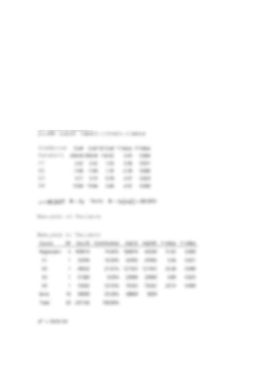
Reserve Problems Chapter 12 Section 2 Problem 1
Consider the following computer output:
(a) Fill in the missing quantities.
The regression equation is
274 2.94 1 3.25 2y x x= + −
Predictor
Coef
SE Coef
T
P
Constant
275.26
6.06
x1
2.9354
0.4949
0
x2
-3.2486
–2.814
3.63685S=
RSq−=
%
( )
RSq adj−=
%
Analysis of Variance
Round your answers to two decimal places (e.g. 98.76).
Source
DF
SS
MS
F
P
Regression
2
684.45
Residual Error
12
130.64
Total
1499.54
(b) What conclusions can you draw about the significance of regression?
(c) What conclusions can you draw about the contributions of the individual regressors to the
model?
SOLUTION
(a)

Reserve Problems Chapter 12 Section 2 Problem 2
Consider the following data:
X1
X2
X3
X4
Y
152.1
32.5
-17
5.833
573.8208
157.9
36
8
3.792
676.1253
106.6
38.9
-6
1.57
421.3201
105.7
42
-26
4.049
395.4186
111.5
40.8
-20
1.394
374.0174
114.7
42.6
-5
0.164
384.9054
116.9
48.2
21
11.432
538.9054
116.2
46.9
26
2.007
450.5508
121.8
53.8
32
1.985
398.2193
122.5
55.4
-20
10.122
508.0602
125.3
56.7
-34
4.087
255.2
123.1
57.4
20
7.529
457.1917
127.7
57.3
-14
15.832
577.3405
124.8
61.4
1
6.857
427.7438
129.3
59.4
-33
11.328
385.4128
130.9
60.5
-2
16.597
588.1741
137.4
66
1
0.628
331.4569
135.1
66.1
0
17.84
386.4599
138.4
69.8
-10
1.178
293.6851
142.1
73.8
11
15.417
346.1528
141.3
75.9
30
18.112
505.4625
(a) Fit a multiple linear regression model to these data. Round constant to nearest whole value.
Estimate
2
.
(b) Test for the significance of regression using
0.05
=
. What is the P-value for this test?
(c) Use the t-test to assess the contribution of each regressor to the model. Using
0.1
=
, and
0.02
=
what conclusions can you draw? What is the P-value for these tests?
SOLUTION
(a)
The computer outflow will be something like the following:
The regression equation is
(b)