Applied Statistics and Probability for Engineers, 7th edition 2017
12-21
(b)
==
2
ˆ9.48
MS
12.2.11 Consider the bearing wear data in Exercise 12.1.13.
(a) For the model with no interaction, test for significance of regression using
= 0.05. What is the P-value for this
test? What are your conclusions?
(b) For the model with no interaction, compute the t-statistics for each regression coefficient. Using
= 0.05, what
conclusion can you draw?
(c) For the model with no interaction, use the extra sum of squares method to investigate the usefulness of adding x2 =
load to a model that already contains x1 = oil viscosity. Use α = 0.05.
(d) Refit the model with an interaction term. Test for significance of regression using
= 0.05.
(e) Use the extra sum of squares method to determine whether the interaction term contributes significantly to the
model. Use
= 0.05.
(d) Estimate
2 for the interaction model. Compare this to the estimate of
2 from the model in part (a).
Applied Statistics and Probability for Engineers, 7th edition 2017
12-22
Reject H0 for regressor
1. Fail to reject H0 for regressor
2.
(c) SSR(
2 |
1,
0) = 1012
H0:
(d) H0:
1 =
2 =
12 = 0
H1 at least one
j ≠ 0
(e) H0:
12 = 0
H1:
12 ≠ 0
(e) With interaction term:
2
ˆ
= 147.0
12.2.12 Data on National Hockey League team performance were presented in Exercise 12.1.12.
(a) Test the model from this exercise for significance of regression using
= 0.05. What conclusions can you draw?
(b) Use the t-test to evaluate the contribution of each regressor to the model. Does it seem that all regressors are
necessary? Use
= 0.05.
(d) Fit a regression model relating the number of games won to the number of goals for and the number of power play
goals for. Does this seem to be a logical choice of regressors, considering your answer to part (b)? Test this new
model for significance of regression and evaluate the contribution of each regressor to the model using the t-test. Use
α = 0.05.
(a) H0:
j = 0 for all j
H1:
Applied Statistics and Probability for Engineers, 7th edition 2017
(b) H0:
j = 0 for all j
H1:
j ≠ 0 for at least one j
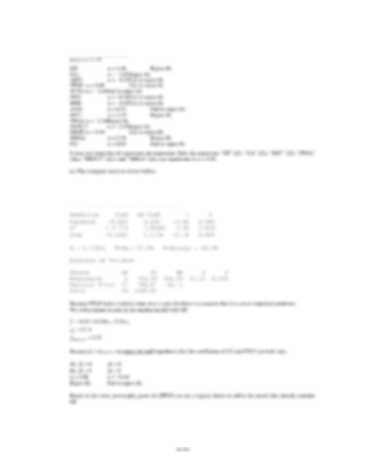
Regression Analysis: W versus GF, PPGF
The regression equation is
W = − 8.82 + 0.218 GF − 0.016 PPGF
12-24
12.2.13 Data from a hospital patient satisfaction survey were presented in Exercise 12.1.5.
(a) Test the model from this exercise for significance of regression. What conclusions can you draw if
= 0.05? What
if
= 0.01?
(b) Test the contribution of the individual regressors using the t-test. Does it seem that all regressors used in the model
are really necessary?
Regression Analysis: Satisfaction versus Age, Severity, Anxiety
The regression equation is
Satisfaction = 144 − 1.11 Age − 0.585 Severity + 1.30 Anxiety
Sections 12-3 and 12-4
12.4.1 Using the regression model from Exercise 12.1.1,
(a) Find a 95% confidence interval for the coefficient of height.
(b) Find a 95% confidence interval for the mean percent of body fat for a man with a height of 72 in. and waist of
34 in.
(c) Find a 95% prediction interval for the percent of body fat for a man with the same height and waist as in part (b).
(d) Which interval is wider, the confidence interval or the prediction interval? Explain briefly.
(e) Given your answer to part (c), do you believe that this is a useful model for predicting body fat? Explain briefly.
Applied Statistics and Probability for Engineers, 7th edition 2017
12-25
(a)
12.4.2 Using the second-order polynomial regression model from Exercise 12.1.2,
(a) Find a 95% confidence interval on both the first-order and the second-order term in this model.
(b) Is zero in the confidence interval you found for the second-order term in part (a)? What does that fact tell you about
the contribution of the second-order term to the model?
(c) Refit the model with only the first-order term. Find a 95% confidence interval on this term. Is this interval longer or
shorter than the confidence interval that you found on this term in part (a)?
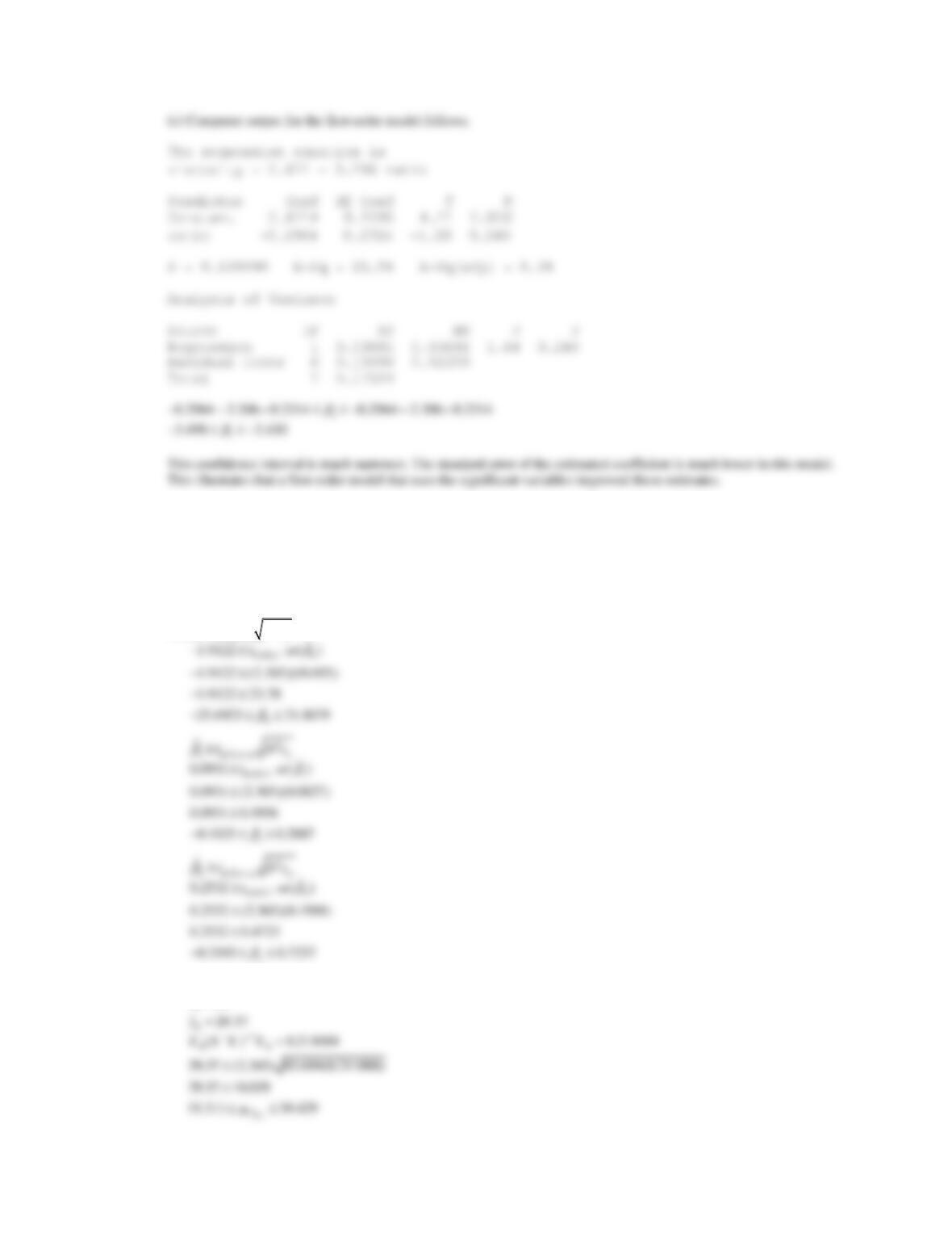
Computer output for the second-order model follows.
The regression equation is
viscosity = 0.198 + 1.37 ratio − 1.28 ratio2
Predictor Coef SE Coef T P
Constant 0.1979 0.4466 0.44 0.676
ratio 1.367 1.488 0.92 0.400
ratio2 −1.280 1.131 −1.13 0.309
S = 0.146606 R-Sq = 37.5% R-Sq(adj) = 12.5%
Analysis of Variance
Source DF SS MS F P
Regression 2 0.06442 0.03221 1.50 0.309
Residual Error 5 0.10747 0.02149
Total 7 0.17189
(a)
==
2.365 for 0.05
t
Applied Statistics and Probability for Engineers, 7th edition 2017
12-26
12.4.3 Consider the soil absorption data in Exercise 12.1.4.
(a) Find 95% confidence intervals on the regression coefficients.
(b) Find a 95% confidence interval on mean soil absorption index when x1 = 200 and x2 = 50.
(c) Find a 95% prediction interval on the soil absorption index when x1 = 200 and x2 = 50.
(a)
−
00
2
0 /2,
ˆˆ
np
tc
−
22
2
2 /2,
ˆˆ
np
tc
(b) x1 = 200
=
50
x
Applied Statistics and Probability for Engineers, 7th edition 2017
12-27
(c)
= 0.05
0
12.4.4 Consider the electric power consumption data in Exercise 12.1.6.
(a) Find 95% confidence intervals on
1,
2,
3, and
4.
(b) Find a 95% confidence interval on the mean of Y when x1 = 75, x2 = 24, x3 = 90, and x4 = 98.
(c) Find a 95% prediction interval on the power consumption when x1 = 75, x2 = 24, x3 = 90, and x4 = 98.
(a) 95% CI on coefficients
0.0973 1.4172
12.4.5 Consider the regression model fit to the X-ray inspection data in Exercise 12.1.7. Use rads as the response.
(a) Calculate 95% confidence intervals on each regression coefficient.
(b) Calculate a 99% confidence interval on mean rads at 15 milliamps and 1 second on exposure time.
(c) Calculate a 99% prediction interval on rads for the same values of the regressors used in the part (b).
(a)
−
11
2
1 /2,
ˆˆ
np
tc
Applied Statistics and Probability for Engineers, 7th edition 2017
12-28
(b)
=−
|
ˆ85.1
Yx
=
|
ˆ
( ) 54.6
Yx
se
t0.005,37 = 2.7154
12.4.6 Consider the wire bond pull strength data in Exercise 12.1.8.
(a) Find 95% confidence interval on the regression coefficients.
(b) Find a 95% confidence interval on mean pull strength when x2 = 20, x3 = 30, x4 = 90, and x5 = 2.0.
(c) Find a 95% prediction interval on pull strength when x2 = 20, x3 = 30, x4 = 90, and x5 = 2.0.
(a)
−
2
0.595 0.535
12.4.7 Consider the regression model fit to the gray range modulation data in Exercise 12.1.11. Use the useful range as the
response.
(a) Calculate 99% confidence intervals on each regression coefficient.
(b) Calculate a 99% confidence interval on mean useful range when brightness = 70 and contrast = 80.
(c) Calculate a prediction interval on useful range for the same values of the regressors used in part (b).
(d) Calculate a 99% confidence interval and a 99% a prediction interval on useful range when brightness = 50 and
contrast = 25. Compare the widths of these intervals to those calculated in parts (b) and (c). Explain any differences in
widths.
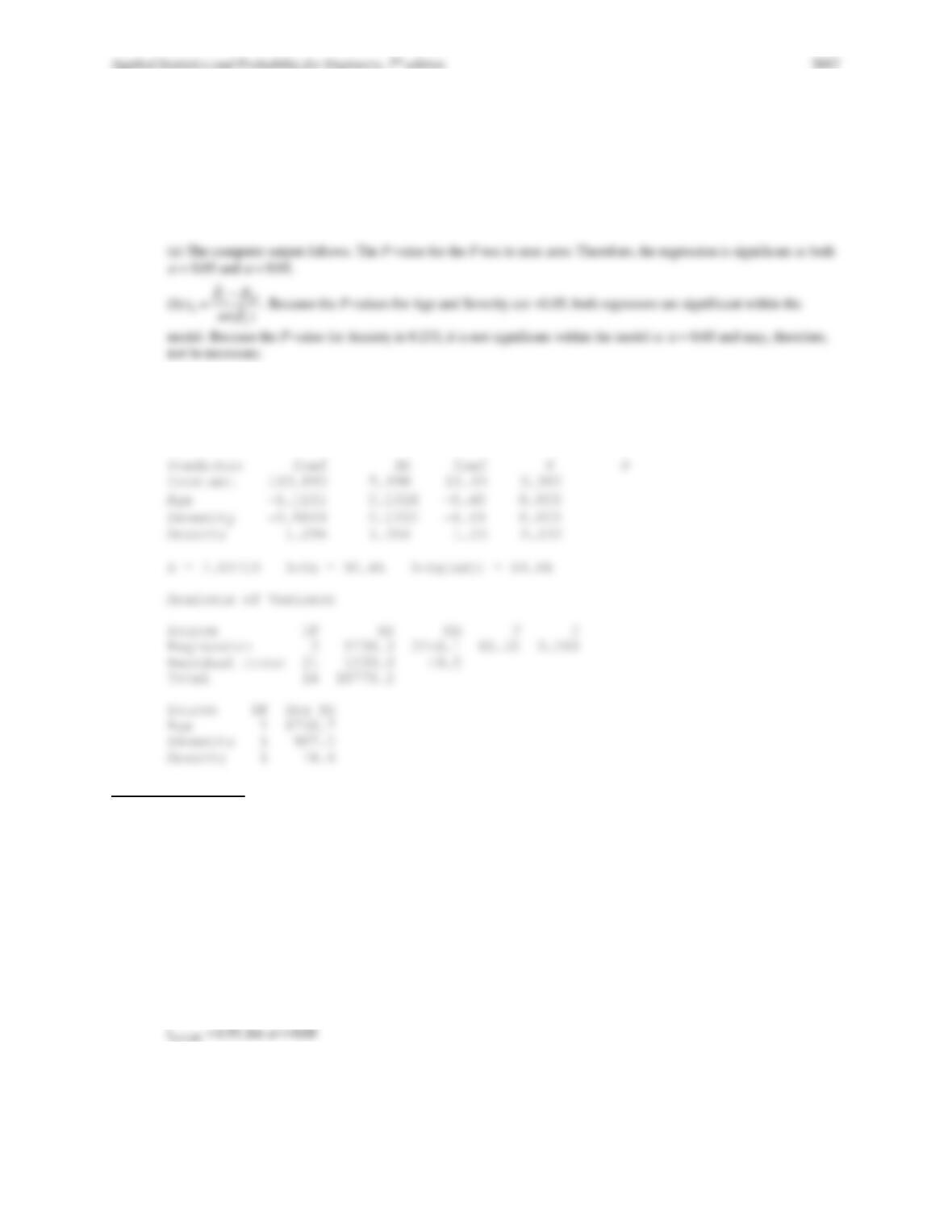
The regression equation is
Useful range (ng) = 239 + 0.334 Brightness (%) − 2.72 Contrast (%)
Predictor Coef SE Coef T P
Constant 238.56 45.23 5.27 0.002
Brightness (%) 0.3339 0.6763 0.49 0.639
Contrast (%) −2.7167 0.6887 −3.94 0.008
S = 36.3493 R-Sq = 75.6% R-Sq(adj) = 67.4%
Analysis of Variance
Source DF SS MS F P
Regression 2 24518 12259 9.28 0.015
Residual Error 6 7928 1321
Total 8 32446
Applied Statistics and Probability for Engineers, 7th edition 2017
(a)
=
0.005,6 3.707t
12.4.8 Consider the regression model fit to the nisin extraction data in Exercise 12.1.10.
(a) Calculate 95% confidence intervals on each regression coefficient.
(b) Calculate a 95% confidence interval on mean nisin extraction when x1 = 15.5 and x2 = 16.
(c) Calculate a prediction interval on nisin extraction for the same values of the regressors used in part (b).
(d) Comment on the effect of a small sample size to the widths of these intervals.
The regression equation is
y = − 171 + 7.03 x1 + 12.7 x2
Predictor Coef SE Coef T P
Constant −171.26 28.40 −6.03 0.001
x1 7.029 1.539 4.57 0.004
x2 12.696 1.539 8.25 0.000
12-30
S = 3.07827 R-Sq = 93.7% R-Sq(adj) = 91.6%
Analysis of Variance
Source DF SS MS F P
Regression 2 842.37 421.18 44.45 0.000
Residual Error 6 56.85 9.48
Total 8 899.22
(a)
−
11
2
1 /2,
ˆˆ
np
tc
1
1
(b)
New
Obs Fit SE Fit 95% CI 95% PI
12.4.9 Consider the NHL data in Exercise 12.1.10.
(a) Find a 95% confidence interval on the regression coefficient for the variable GF.
(b) Fit a simple linear regression model relating the response variable to the regressor GF.
(c) Find a 95% confidence interval on the slope for the simple linear regression model from part (b).
(d) Compare the lengths of the two confidence intervals computed in parts (a) and (c). Which interval is shorter? Does
this tell you anything about which model is preferable?
(a) From the computer output, the estimate, standard error, t statistic and P-value for the coefficient of GF are
Predictor Coef SE Coef T P
Applied Statistics and Probability for Engineers, 7th edition 2017
12-31
Applied Statistics and Probability for Engineers, 7th edition 2017
12-32
Section 12.5
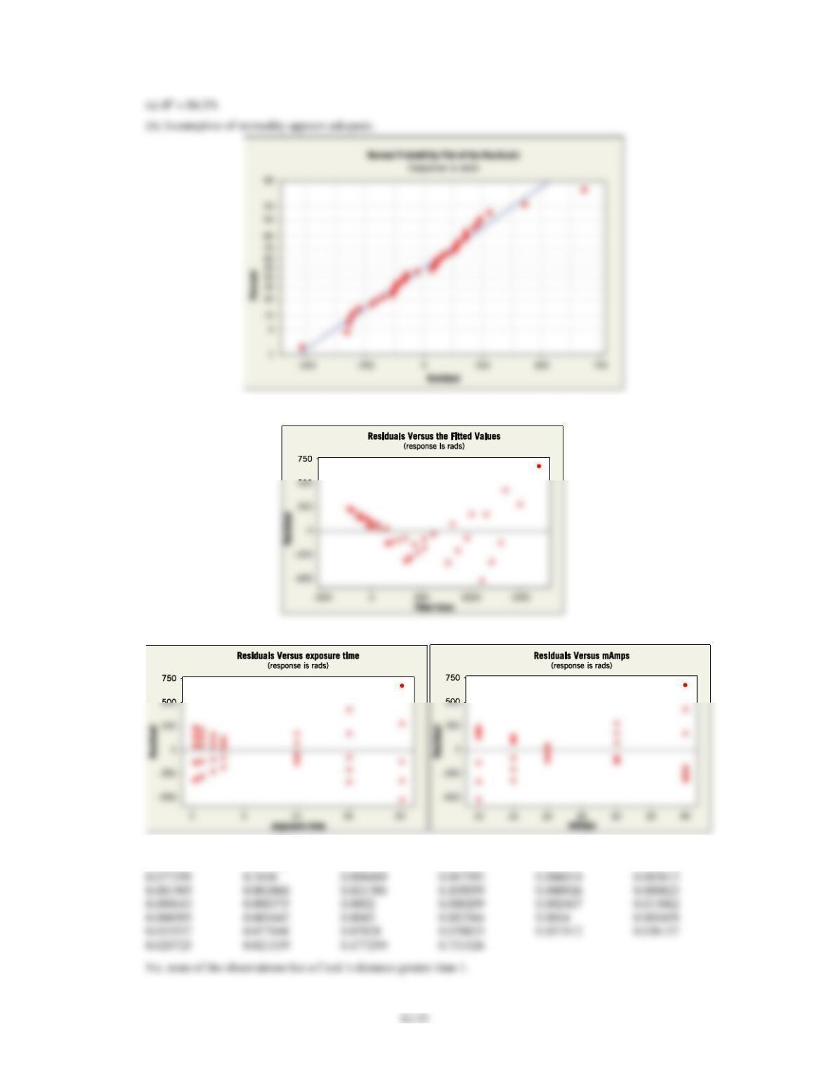
12.5.1 Consider the regression model fit to the X-ray inspection data in Exercise 12.1.7. Use rads as the response.
(a) What proportion of total variability is explained by this model?
(b) Construct a normal probability plot of the residuals. What conclusion can you draw from this plot?
(c) Plot the residuals versus
ˆ
y
and versus each regressor, and comment on model adequacy.
(d) Calculate Cook’s distance for the observations in this data set. Are there any influential points in these data?
Applied Statistics and Probability for Engineers, 7th edition 2017
(c) There are funnel shapes in the graphs, so the assumption of constant variance is violated. The model is inadequate.
(d) Cook’s distance values
0.032728 0.029489 0.023724 0.014663 0.008279 0.008611
12-34
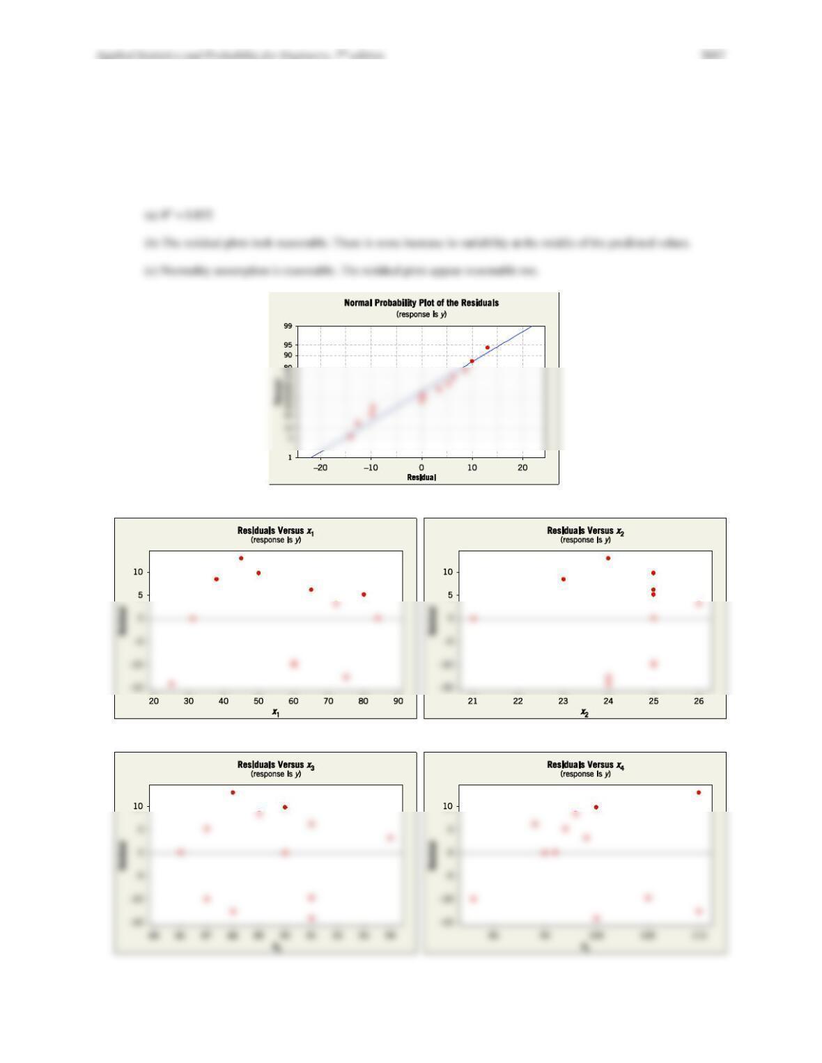
12.5.2 Consider the electric power consumption data in Exercise 12.5.2.
(a) Calculate R2 for this model. Interpret this quantity.
(b) Plot the residuals versus
ˆ
y
and versus each regressor. Interpret this plot.
(c) Construct a normal probability plot of the residuals and comment on the normality assumption.
Applied Statistics and Probability for Engineers, 7th edition 2017
12-35
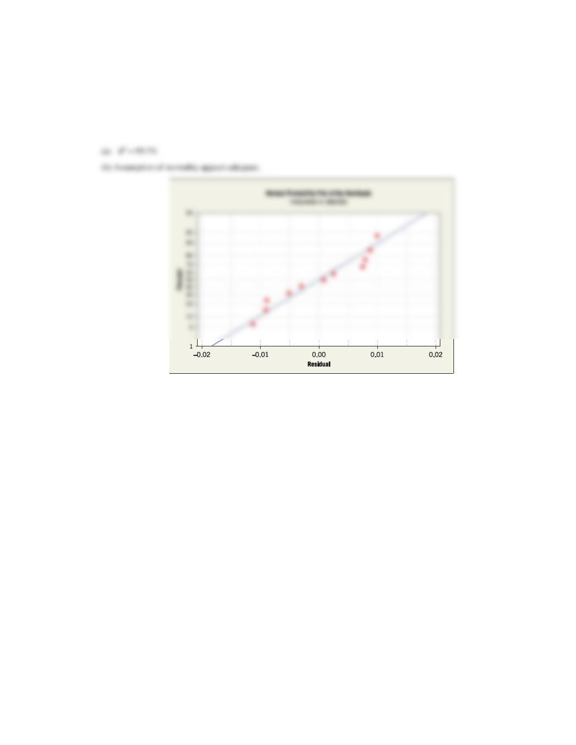
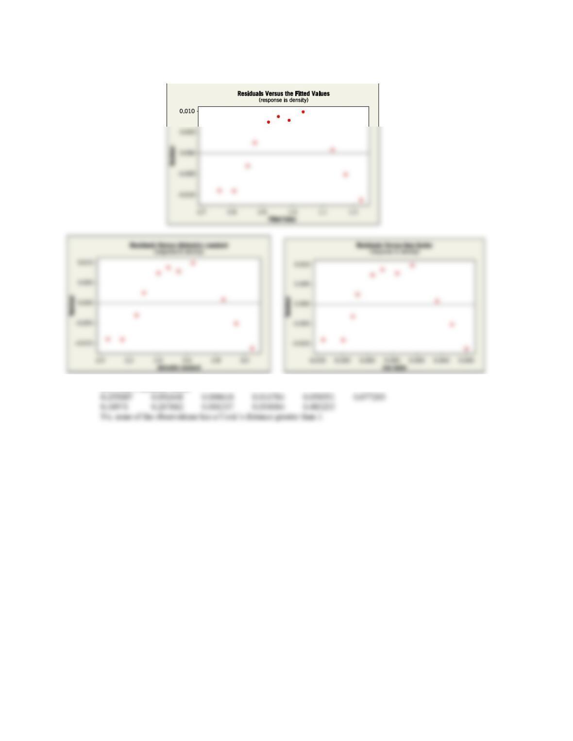
12.5.3 Consider the regression model fit to the coal and limestone mixture data in Exercise 12.1.9. Use density as the
response.
(a) What proportion of total variability is explained by this model?
(b) Construct a normal probability plot of the residuals. What conclusion can you draw from this plot?
(c) Plot the residuals versus
ˆ
y
and versus each regressor, and comment on model adequacy.
(d) Calculate Cook’s distance for the observations in this data set. Are there any influential points in these data?
Applied Statistics and Probability for Engineers, 7th edition 2017
12-36
(c) There is a nonconstant variance shown in graphs. Therefore, the model is inadequate.
(d) Cook’s distance values
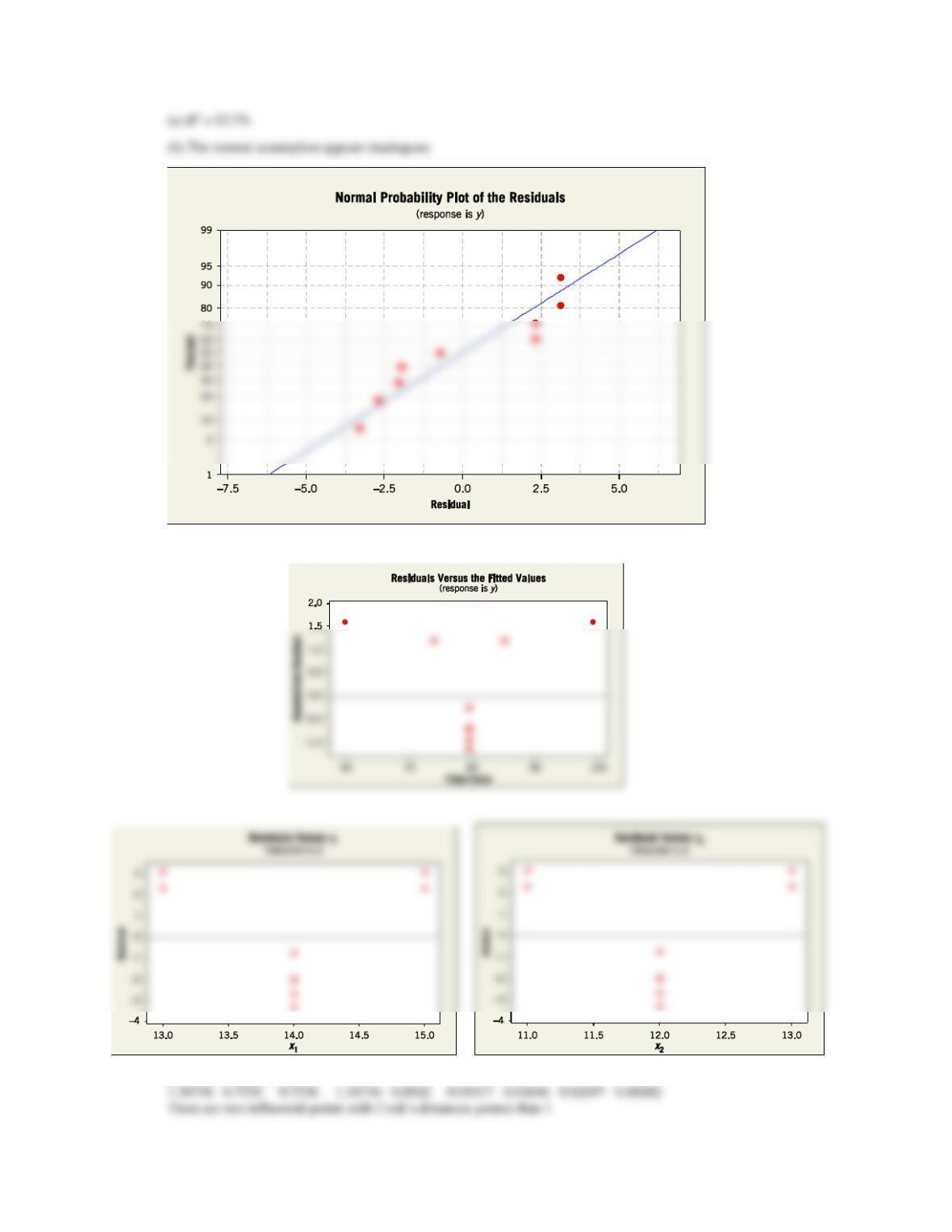
12.5.4 Consider the regression model fit to the nisin extraction data in Exercise 12.1.10.
(a) What proportion of total variability is explained by this model?
(b) Construct a normal probability plot of the residuals. What conclusion can you draw from this plot?
(c) Plot the residuals versus
ˆ
y
and versus each regressor, and comment on model adequacy.
(d) Calculate Cook’s distance for the observations in this data set. Are there any influential points in these data?
Applied Statistics and Probability for Engineers, 7th edition 2017
12-37
(c) The constant variance assumption is not valid.
(d) Cook’s distance values
Applied Statistics and Probability for Engineers, 7th edition 2017
12-38
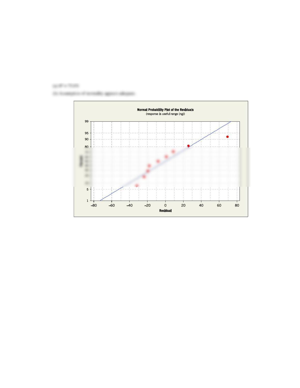
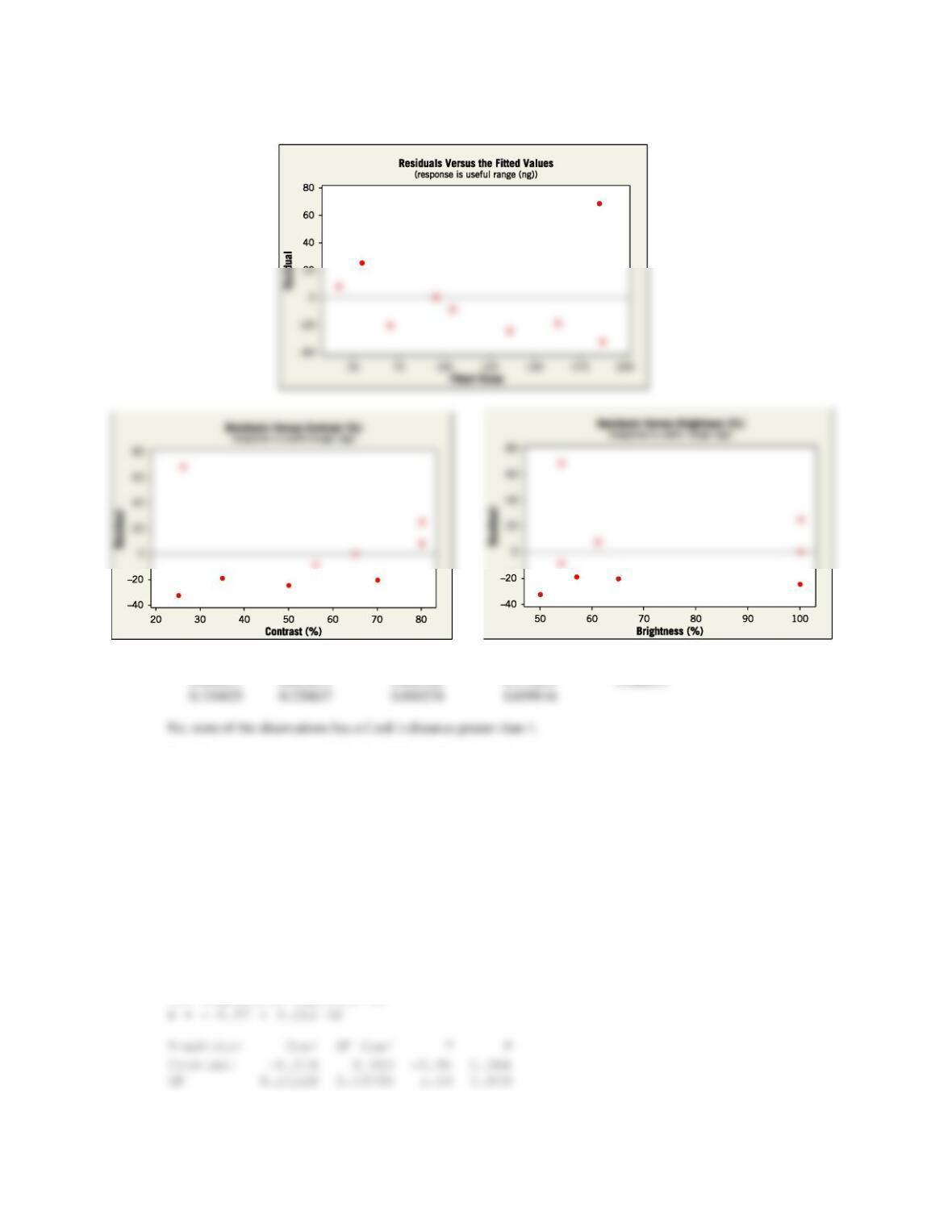
12.5.5 Consider the regression model fit to the gray range modulation data in Exercise 12.1.11. Use the useful range as the
response.
(a) What proportion of total variability is explained by this model?
(b) Construct a normal probability plot of the residuals. What conclusion can you draw from this plot?
(c) Plot the residuals versus
ˆ
y
and versus each regressor, and comment on model adequacy.
(d) Calculate Cook’s distance for the observations in this data set. Are there any influential points in these data?
Applied Statistics and Probability for Engineers, 7th edition 2017
12-39
(c) Assumption of constant variance is a possible concern. One point is a concern as a possible outlier.
(d) Cook’s distance values
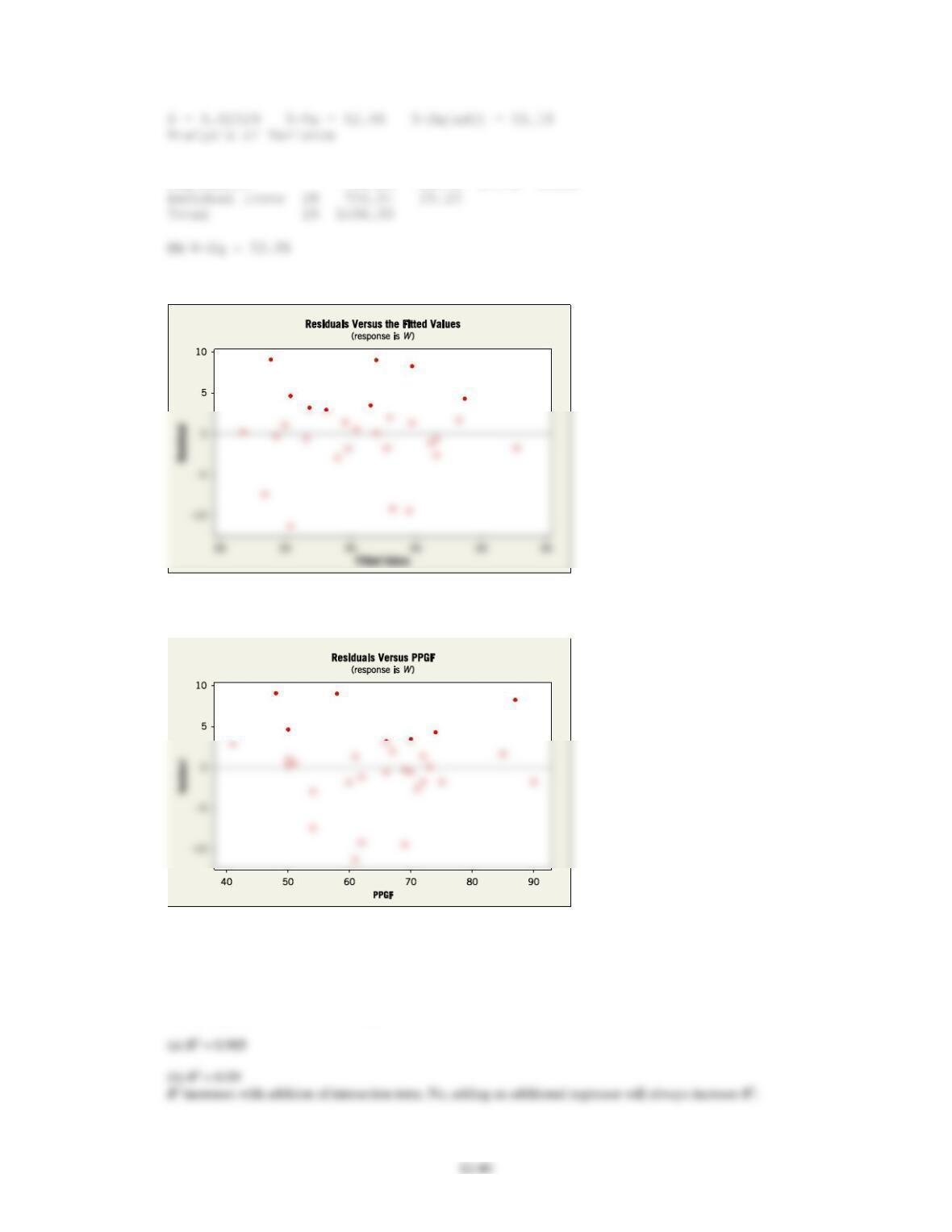
12.5.6 Consider the regression model for the NHL data from Exercise 12.1.12.
(a) Fit a model using GF as the only regressor.
(b) How much variability is explained by this model?
(c) Plot the residuals versus
ˆ
y
and comment on model adequacy.
(d) Plot the residuals from part (a) versus PPGF, the points scored while in power play. Does this indicate that the
model would be better if this variable were included?
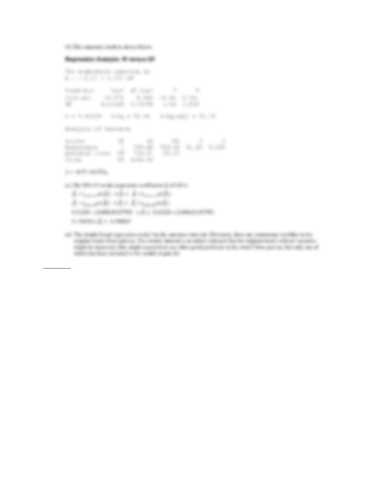
(a) The computer output is shown below.
Regression Analysis: W versus GF
The regression equation is
Applied Statistics and Probability for Engineers, 7th edition 2017
Source DF SS MS F P
Regression 1 789.46 789.46 31.29 0.000
(c) Model appears adequate.
(d) No, the residuals do not seem to be related to PPGF. Because there is no pattern evident in the plot, it does not seem
that this variable would contribute significantly to the model.
12.5.7 Consider the bearing wear data in Exercise 12.1.13.
(a) Find the value of R2 when the model uses the regressors x1 and x2.
(b) What happens to the value of R2 when an interaction term x1x2 is added to the model? Does this necessarily imply
that adding the interaction term is a good idea?