(b) Calculate a 95% confidence interval on mean stack loss when
180x=
,
220x=
, and
390x=
.
(c) Calculate a 95% prediction interval on stack loss for the same values of the regressors used in
part (b).
(d) Calculate a 95% confidence interval and a 95% prediction interval on stack loss when
180x=
,
214x=
, and
393x=
.
Compare the widths of these intervals to those calculated in parts (b) and (c). Explain any
differences in widths.
These part (d) intervals are ______ because the regressors are set at extreme values in the x space
and the standard errors are _______.
SOLUTION
Predictor
Coef
SE Coef
Constant
-39.920
11.896
(a) A
( )
100 1 %
−
confidence interval on the regression coefficient
j
is
(b) A
( )
100 1 %
−
confidence interval on the mean response is
( )
100 1 %
−
(d) Prediction at
180x=
,
214x=
, and
393x=
is
0
|21.3540
ˆYx
=

Reserve Problems Chapter 12 Section 5 Problem 1
The table presents the values of Human Development Index (y), life expectancy (
1
x
, in years),
and food energy intake (
2
x
, in kcal per capita per day) for 16 countries.
No
Country
HDI, y
Life expectancy,
1
x
Food energy intake,
2
x
1
Argentina
0.827
76.3
3030
2
Belarus
0.796
72.3
3150
3
Belgium
0.896
81.1
3690
4
Brazil
0.754
75.0
3120
5
Denmark
0.925
80.6
3410
6
Egypt
0.691
70.9
3160
7
Finland
0.895
81.1
3220
8
France
0.897
82.4
3530
9
Germany
0.926
81.0
3540
10
Greece
0.866
81.0
3710
11
Hungary
0.836
75.9
3470
12
Italy
0.887
82.7
3650
13
Turkey
0.767
75.8
3500
14
Ukraine
0.743
71.3
3290
15
United Kingdom
0.909
81.2
3450
16
USA
0.920
79.3
3750
a) Fit a multiple linear regression model to these data. Estimate the parameters in the model
0 1 1 2 2
Y x x
= + + +
.
What proportion of the total variability is explained by this model?
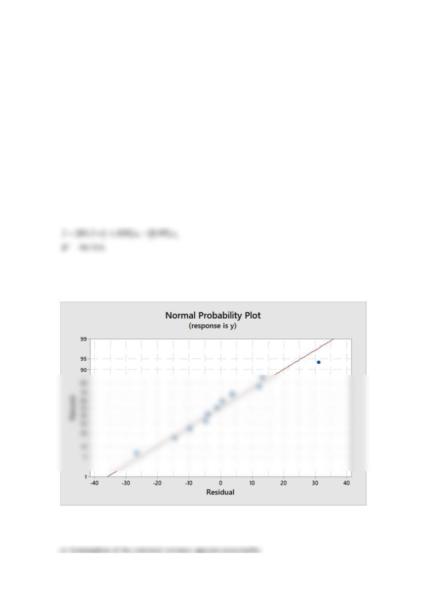
b) Construct a normal probability plot of the residuals. Does the assumption of normality appear
adequate?
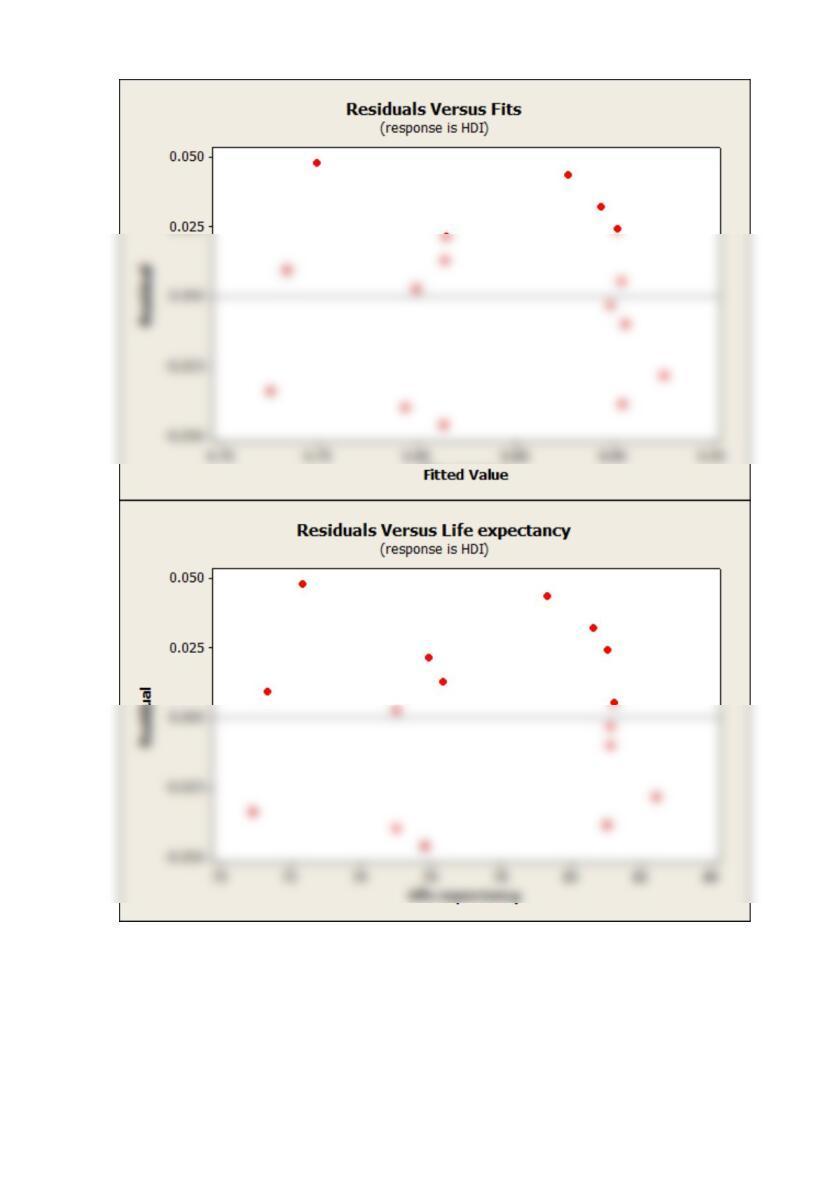
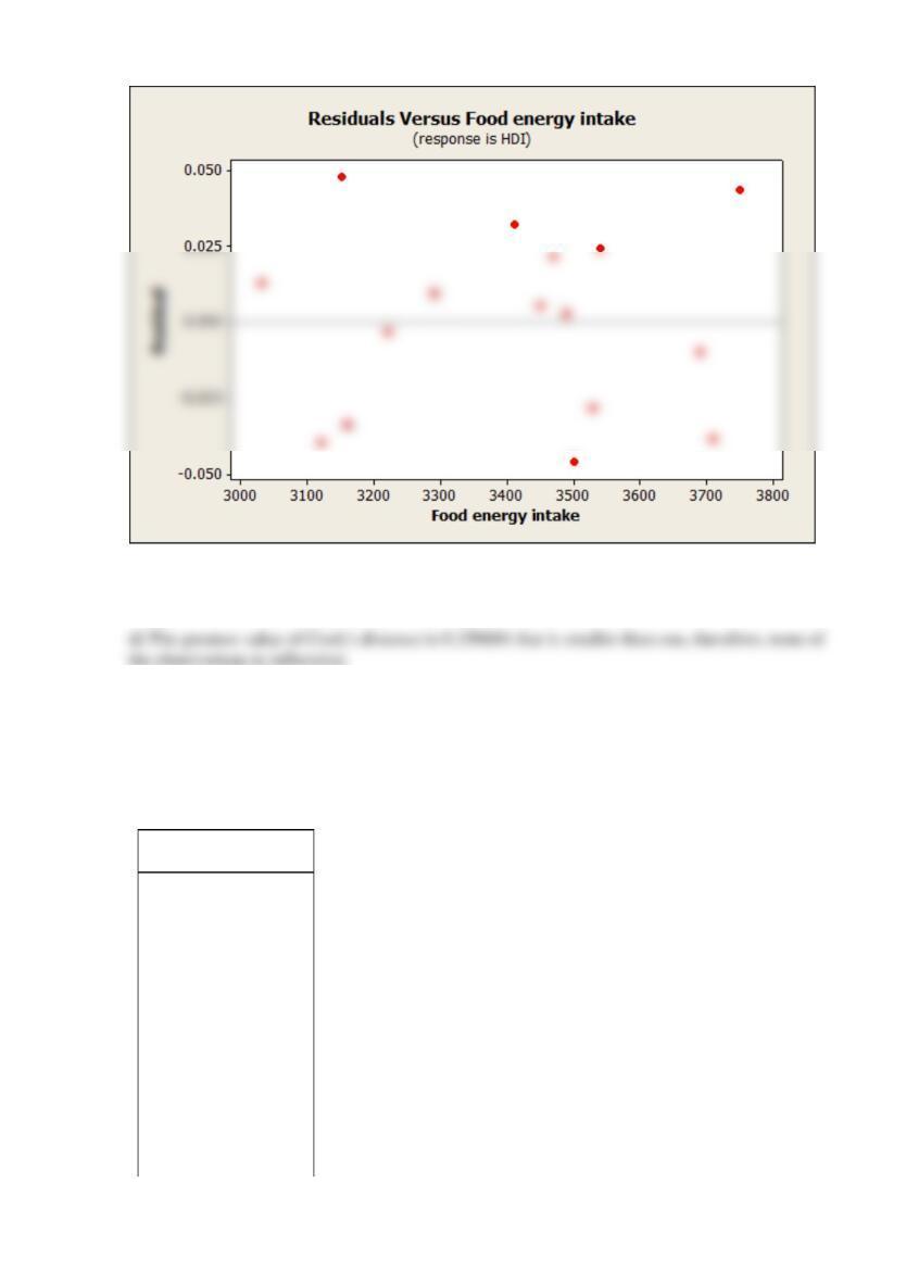
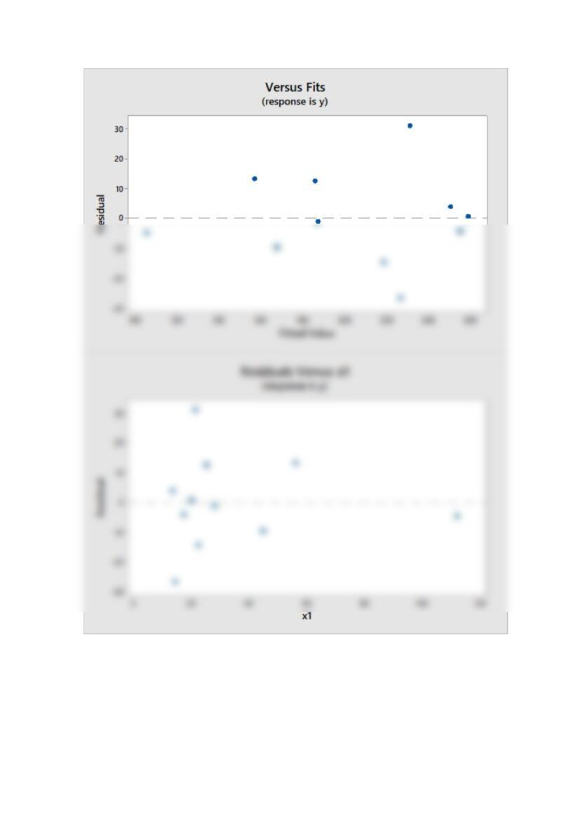
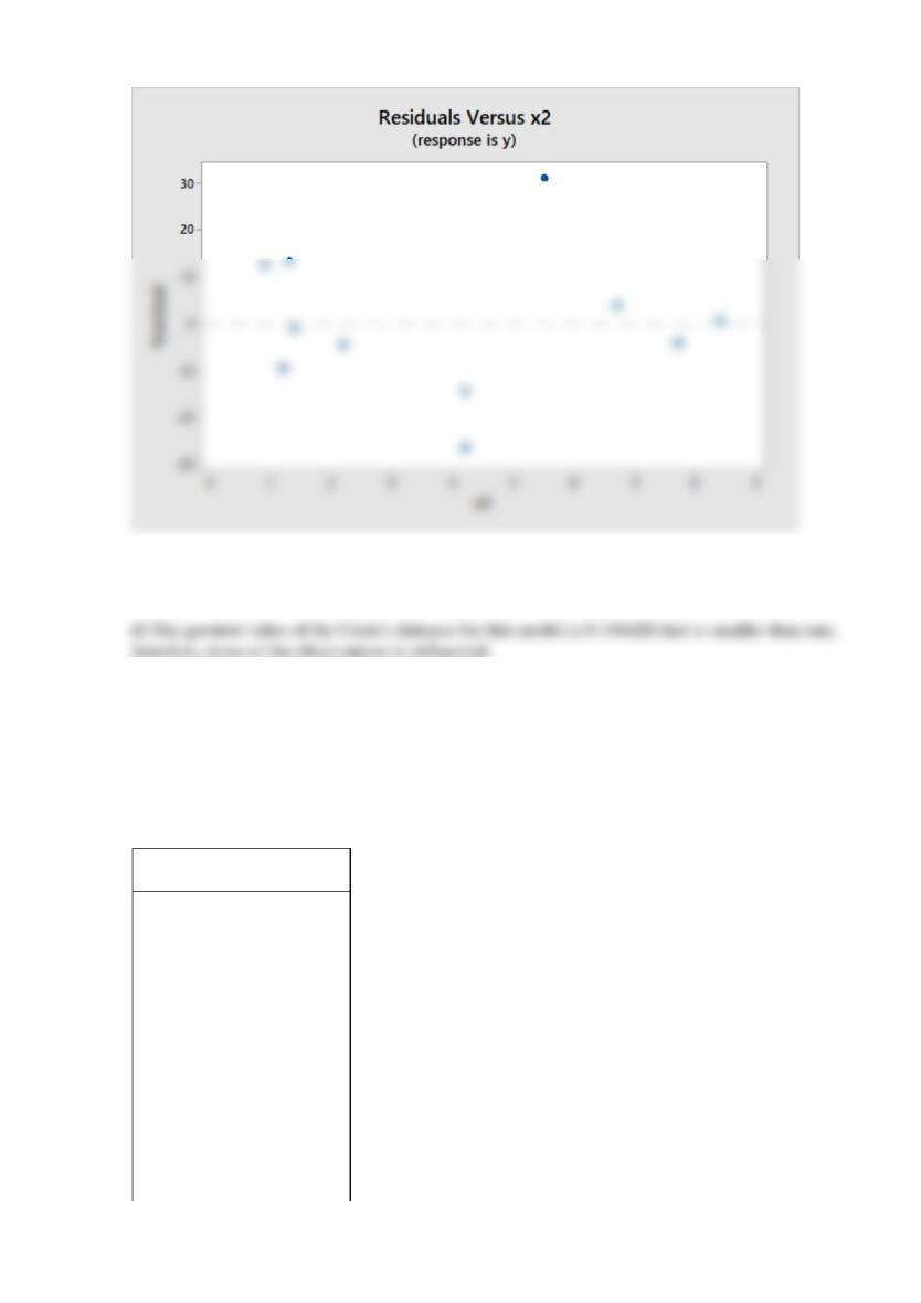
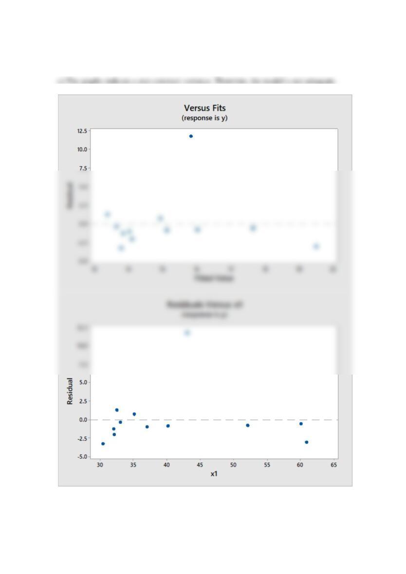
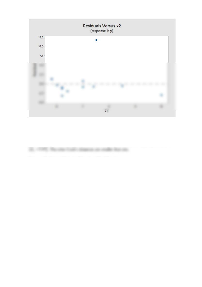
b) Plot the residuals versus fitted values and versus each regressor. Does the assumption of the
constant variance seem reasonable?
d) Calculate Cook’s distance values for the observations in this data set. Are any observations
influential?
SOLUTION
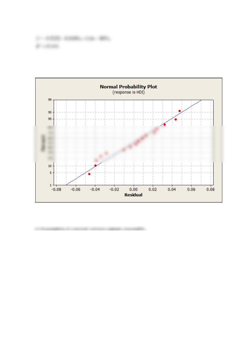
a) The regression equation is
b) Assumption of normality appears adequate.
Reserve Problems Chapter 12 Section 5 Problem 2
Data on coal production per worker (y, in tons), coal bed thickness (
1
x
, in meters), and the level
of the mechanization (
2
x
, in percent), characterizing the process of coal mining in 10 mines are
given in the following table.
No
y
1
x
2
x
1
5
8
5
2
10
11
8
3
10
12
8
4
7
9
5
5
5
8
7
6
6
8
8
7
6
9
6
8
5
9
4
9
6
8
5
10
8
12
7
a) Fit a multiple linear regression model to these data.
Calculate
2
R
for this model.
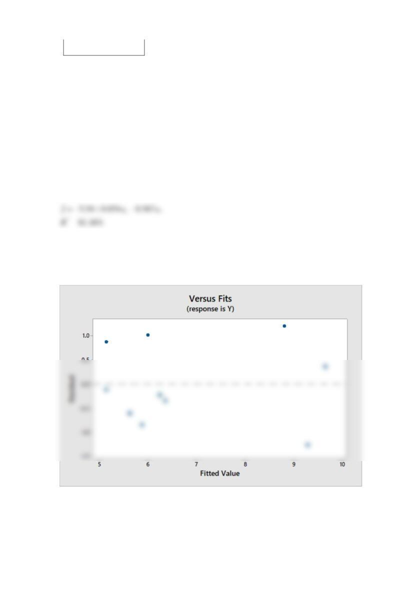
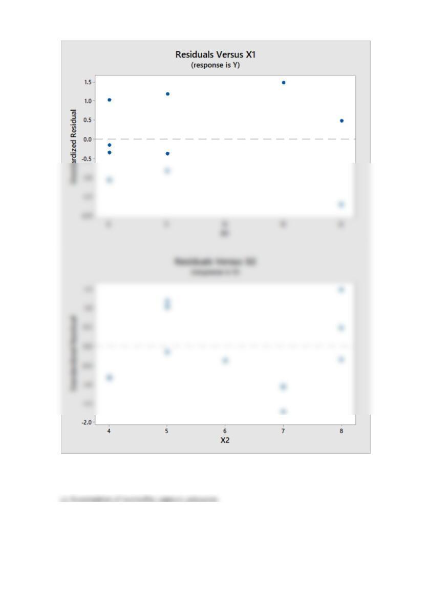
b) Plot the residuals versus fitted values and versus each regressor. Does the assumption of
constant variance seem reasonable?
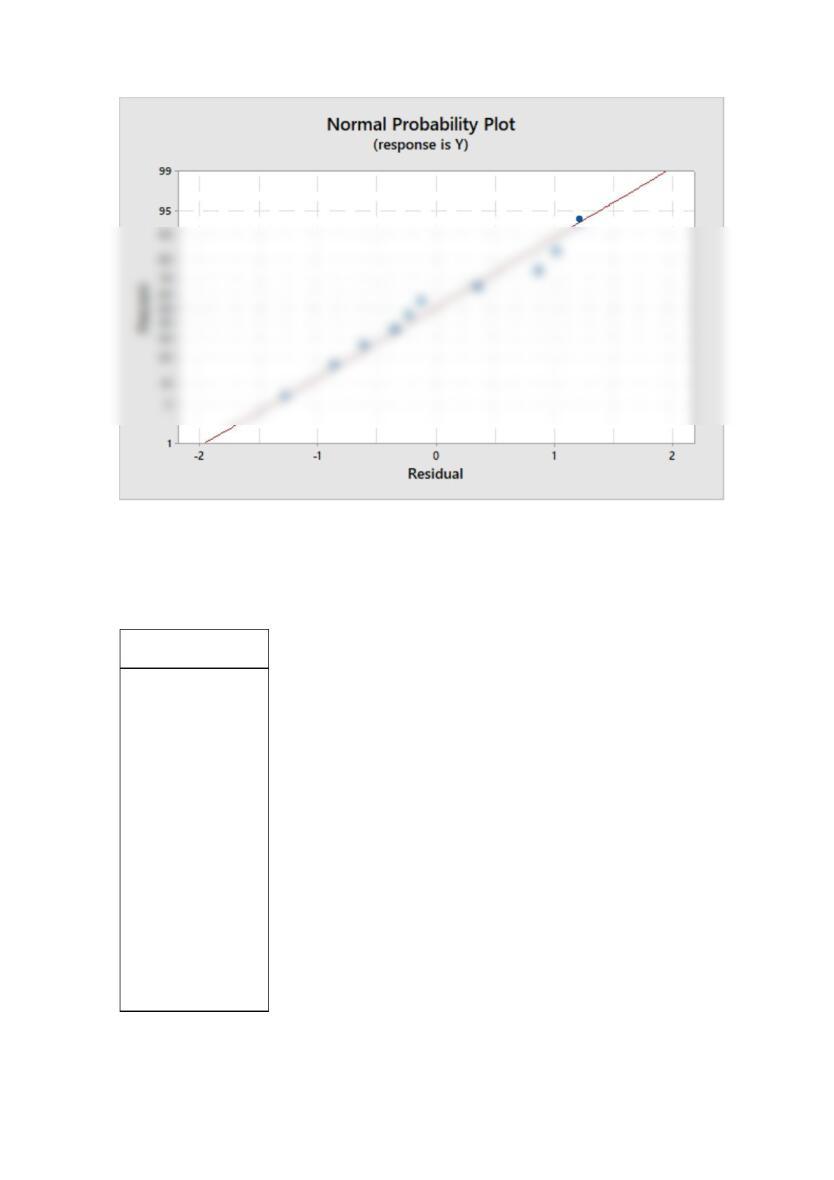
c) Construct a normal probability plot of the residuals. Does the assumption of normality appear
adequate?
SOLUTION
a) The regression equation is
b) Assumption of the constant variable appears reasonable.
Reserve Problems Chapter 12 Section 5 Problem 3
Data on the cost of one ton of steel (y), production of steel per worker (
1
x
, in tons), and defect
percentage (
2
x
) are given in the table.
y
1
x
2
x
200
14.6
4.2
254
13.5
6.7
262
21.5
5.5
251
17.4
7.7
158
44.8
1.2
101
111.9
2.2
259
20.1
8.4
186
28.1
1.4
204
22.3
4.2
198
25.3
0.9
170
56.0
1.3
a) Fit a multiple linear regression model to these data. What proportion of the total variability is
explained by this model?
b) Construct a normal probability plot of the residuals. Does the assumption of normality appear
adequate?
c) Plot the residuals versus fitted values and versus each regressor. Does the assumption of
constant variance seem reasonable?
d) Calculate Cook’s distance values for the observations in this data set. Are any observations
influential?
SOLUTION
a) The regression equation is
b) Assumption of normality appears adequate.
Reserve Problems Chapter 12 Section 5 Problem 4
The following table shows data on the secondary housing market in a district of a city: the cost
of the apartment (y, in thousand USD), the size of the living space (
1
x
, in m2), and the size of the
kitchen (
2
x
, in m2).
No
y
1
x
2
x
1
13.0
37.0
6.2
2
16.4
60.9
10.0
3
17.0
60.0
8.5
4
15.2
52.1
7.4
5
14.2
40.1
7.0
6
10.5
30.4
6.2
7
27.5
43.0
7.5
8
12.0
32.1
6.4
9
15.6
35.1
7.0
10
12.5
32.0
6.2
11
13.2
33.0
6.0
12
14.6
32.5
5.8
a) Fit a multiple linear regression model to these data.
Calculate
2
R
for this model.
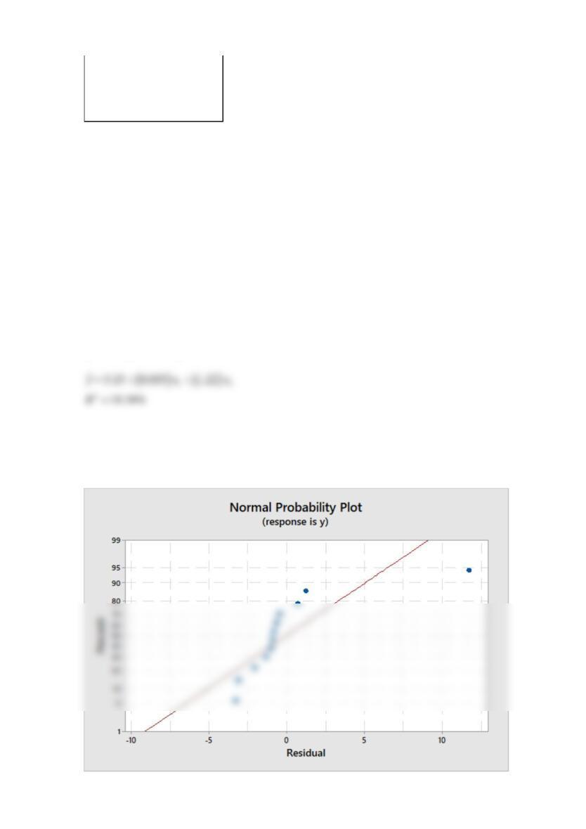
b) Construct a normal probability plot of the residuals. Does the assumption of normality appear
adequate?
c) Plot the residuals versus fitted values and versus each regressor. Does the assumption of
constant variance seem reasonable?
d) Calculate Cook’s distance values for the observations in this data set. Are any observations
influential?
SOLUTION
a) The regression equation is
b) Assumption of normality appears inadequate.
d) There is one influential point (the second one) with Cook’s distance greater than one
Reserve Problems Chapter 12 Section 5 Problem 5

Table given below provides the highway gasoline mileage test results for 2005 model year vehicles from DaimlerChrysler.
mf
r
carline
car/
truck
cid
rhp
trn
s
dr
v
o
d
etw
cm
p
axle
n/v
a/
c
hc
co
co2
mpg
20
300C/SRT-8
C
21
5
25
3
L5
4
2
450
0
9.9
3.0
7
30.
9
Y
0.01
1
0.0
9
28
8
30.8
20
CARAVAN 2WD
T
20
1
18
0
L4
F
2
450
0
9.3
2.4
9
32.
3
Y
0.01
4
0.1
1
27
4
32.5
20
CROSSFIRE ROADSTER
C
19
6
16
8
L5
R
2
337
5
10
3.2
7
37.
1
Y
0.00
1
0.0
2
25
0
37.6
20
DAKOTA PICKUP 2WD
T
22
6
21
0
L4
R
2
450
0
9.2
3.5
5
29.
6
Y
0.01
2
0.0
4
31
6
28.1
20
DAKOTA PICKUP 4WD
T
22
6
21
0
L4
4
2
500
0
9.2
3.5
5
29.
6
Y
0.01
1
0.0
5
36
5
24.4
20
DURANGO 2WD
T
34
8
34
5
L5
R
2
525
0
8.6
3.5
5
27.
2
Y
0.02
3
0.1
5
36
7
24.1
20
GRAND CHEROKEE 2WD
T
22
6
21
0
L4
R
2
450
0
9.2
3.0
7
30.
4
Y
0.00
6
0.0
9
31
2
31.8
20
GRAND CHEROKEE 4WD
T
34
8
23
0
L5
4
2
500
0
9
3.0
7
24.
7
Y
0.00
8
0.1
1
36
9
24.2
20
LIBERTY/CHEROKEE
2WD
T
14
8
15
0
M6
R
2
400
0
9.5
4.1
41
Y
0.00
4
0.4
1
27
0
33.9
20
LIBERTY/CHEROKEE
4WD
T
22
6
21
0
L4
4
2
425
0
9.2
3.7
3
31.
2
Y
0.00
3
0.0
4
31
7
28.0
20
NEON/SRT-4/SX 2
C
12
2
13
2
L4
F
2
300
0
9.8
2.6
9
39.
2
Y
0.00
3
0.1
6
21
4
46.8
20
PACIFICA 2WD
T
21
5
24
9
L4
F
2
475
0
9.9
2.9
5
35.
3
Y
0.02
2
0.0
1
29
5
30.0
20
PACIFICA AWD
T
21
5
24
9
L4
4
2
500
0
9.9
2.9
5
35.
3
Y
0.02
4
0.0
5
31
4
28.2
20
PT CRUISER
T
14
8
22
0
L4
F
2
362
5
9.5
2.6
9
37.
3
Y
0.00
2
0.0
3
26
0
33.0
20
RAM 1500 PICKUP 2WD
T
50
0
50
0
M6
R
2
525
0
9.6
4.1
22.
3
Y
0.01
0.1
47
4
18.7
20
RAM 1500 PICKUP 4WD
T
34
8
34
5
L5
4
2
600
0
8.6
3.9
2
29
Y
0
0
0
20.3
20
SEBRING 4-DR
C
16
5
20
0
L4
F
2
362
5
9.7
2.6
9
36.
8
Y
0.01
1
0.1
2
25
2
40.6
20
STRATUS 4-DR
C
14
8
16
7
L4
F
2
350
0
9.5
2.6
9
36.
8
Y
0.00
2
0.0
6
23
3
37.9
20
TOWN & COUNTRY 2WD
T
14
8
15
0
L4
F
2
425
0
9.4
2.6
9
34.
9
Y
0
0.0
9
26
2
39.3
20
VIPER CONVERTIBLE
C
50
0
50
1
M6
R
2
375
0
9.6
3.0
7
19.
4
Y
0.00
7
0.0
5
34
2
25.9
20
WRANGLER/TJ 4WD
T
14
8
15
0
M6
4
2
362
5
9.5
3.7
3
40.
1
Y
0.00
4
0.4
3
33
7
26.4
Consider a multiple linear regression model to these data to estimate gasoline mileage (mpg) that uses the following regressors: cid, rhp, etw, cmp,
axle, n/v.
(a) What proportion of total variability is explained by this model?
(b) Calculate Cook’s distance for the observations in this data set. Are any observations
influential?
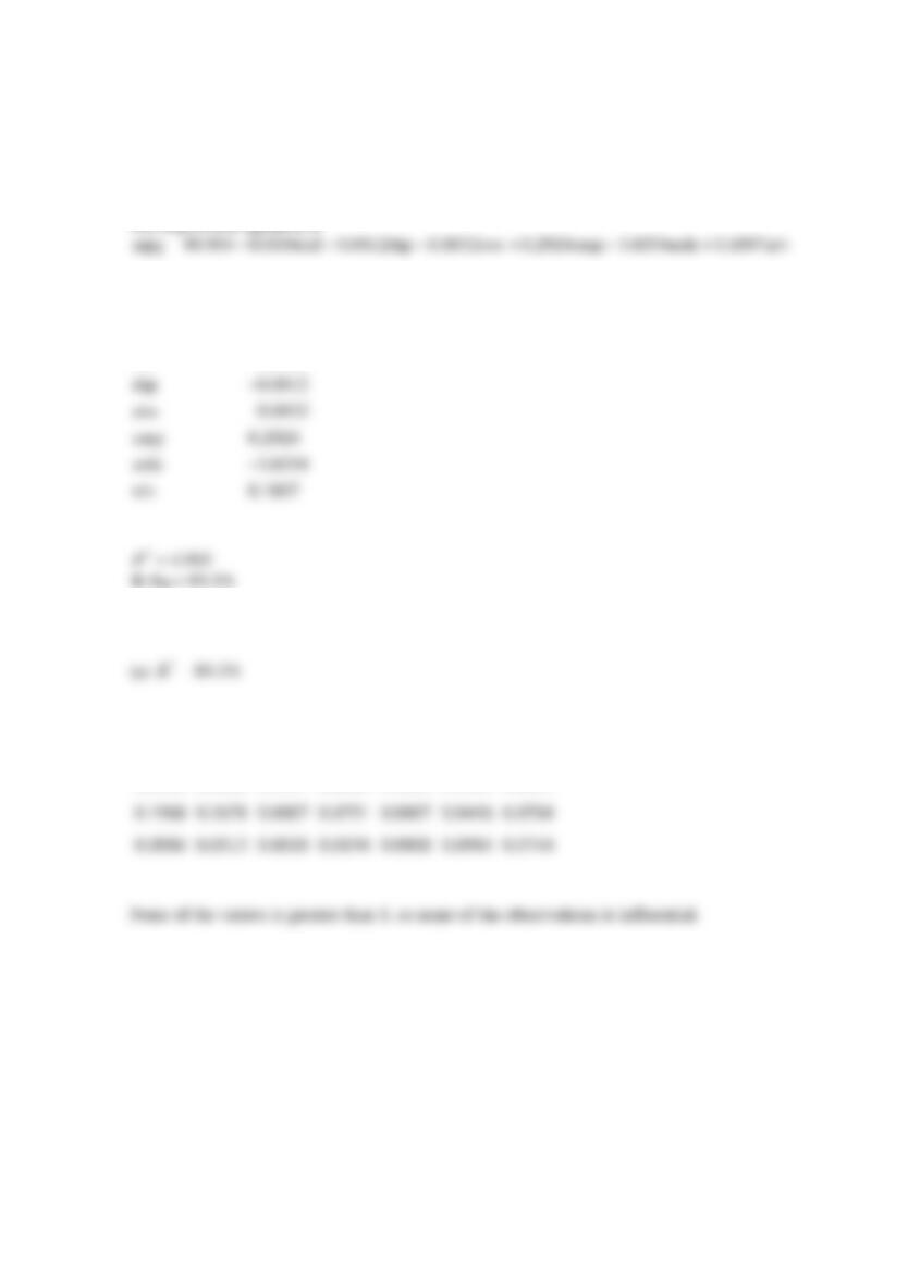
SOLUTION
Predictor
Coef
Constant
49.904
cid
–0.0104
rhp
–0.0012
etw
–0.0032
cmp
0.2924
axle
–3.8554
n/v
0.1897
(b) Cook’s distance values
0.0362
0.0006
0.0417
0.0085
0.0268
0.0404
0.0031
0.1968
0.2678
0.0007
0.0751
0.0007
0.0416
0.0704
0.0086
0.0513
0.0018
0.0194
0.0008
0.0984
0.5744
Reserve Problems Chapter 12 Section 5 Problem 6
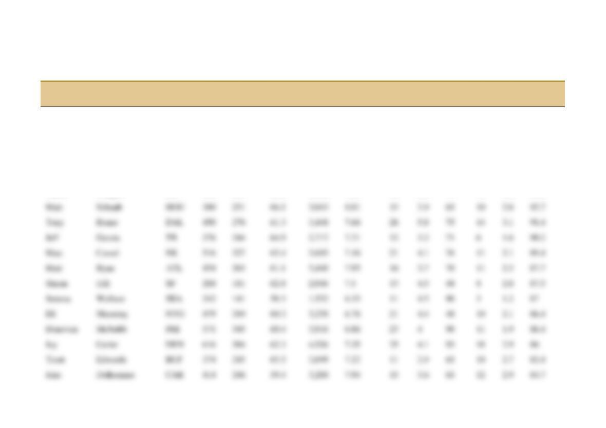
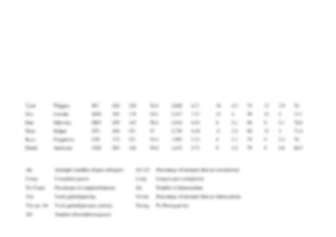
Table given below presents quarterback ratings for the 2008 National Football League season (The Sports Network). Consider a multiple regression
model to relate the quarterback rating to the percentage of completions, the percentage of TDs, and the percentage of interceptions.
Player
Team
Att
Comp
Pct
Comp
Yds
Yds per
Att
TD
Pct
TD
Lng
Int
Pct
Int
Rating
Pts
Philip
Rivers
SD
478
312
65.3
4,009
8.39
34
7.1
67
11
2.3
105.5
Chad
Pennington
MIA
476
321
67.4
3,653
7.67
19
4
80
7
1.5
97.4
Kurt
Warner
ARI
598
401
67.1
4,583
7.66
30
5
79
14
2.3
96.9
Drew
Brees
NO
635
413
65
5,069
7.98
34
5.4
84
17
2.7
96.2
Peyton
Manning
IND
555
371
66.8
4,002
7.21
27
4.9
75
12
2.2
95
Aaron
Rodgers
GB
536
341
63.6
4,038
7.53
28
5.2
71
13
2.4
93.8
Matt
Schaub
HOU
380
251
66.1
3,043
8.01
15
3.9
65
10
2.6
92.7
Tony
Romo
DAL
450
276
61.3
3,448
7.66
26
5.8
75
14
3.1
91.4
Jeff
Garcia
TB
376
244
64.9
2,712
7.21
12
3.2
71
6
1.6
90.2
Matt
Cassel
NE
516
327
63.4
3,693
7.16
21
4.1
76
11
2.1
89.4
Matt
Ryan
ATL
434
265
61.1
3,440
7.93
16
3.7
70
11
2.5
87.7
Shaun
Hill
SF
288
181
62.8
2,046
7.1
13
4.5
48
8
2.8
87.5
Seneca
Wallace
SEA
242
141
58.3
1,532
6.33
11
4.5
90
3
1.2
87
Eli
Manning
NYG
479
289
60.3
3,238
6.76
21
4.4
48
10
2.1
86.4
Donovan
McNabb
PHI
571
345
60.4
3,916
6.86
23
4
90
11
1.9
86.4
Cutler
DEN
616
384
62.3
4,526
7.35
25
4.1
93
18
2.9
86
Jason
Campbell
WAS
506
315
62.3
3,245
6.41
13
2.6
67
6
1.2
84.3
David
Garrard
JAC
535
335
62.6
3,620
6.77
15
2.8
41
13
2.4
81.7
Brett
Favre
NYJ
522
343
65.7
3,472
6.65
22
4.2
56
22
4.2
81
Joe
Flacco
BAL
428
257
60
2,971
6.94
14
3.3
70
12
2.8
80.3
Kerry
Collins
TEN
415
242
58.3
2,676
6.45
12
2.9
56
7
1.7
80.2
Ben
Roethlisberger
PIT
469
281
59.9
3,301
7.04
17
3.6
65
15
3.2
80.1
Kyle
Orton
CHI
465
272
58.5
2,972
6.39
18
3.9
65
12
2.6
79.6
JaMarcus
Russell
OAK
368
198
53.8
2,423
6.58
13
3.5
84
8
2.2
77.1
Tyler
Thigpen
KC
420
230
54.8
2,608
6.21
18
4.3
75
12
2.9
76
Gus
Frerotte
MIN
301
178
59.1
2,157
7.17
12
4
99
15
5
73.7
Dan
Orlovsky
DET
255
143
56.1
1,616
6.34
8
3.1
96
8
3.1
72.6
Marc
Bulger
STL
440
251
57
2,720
6.18
11
2.5
80
13
3
71.4
Ryan
Fitzpatrick
CIN
372
221
59.4
1,905
5.12
8
2.2
79
9
2.4
70
Derek
Anderson
CLE
283
142
50.2
1,615
5.71
9
3.2
70
8
2.8
66.5
Att
Attempts (number of pass attempts)
Pct TD
Percentage of attempts that are touchdowns
Comp
Completed passes
Long
Longest pass completion
Pct Comp
Percentage of completed passes
Int
Number of interceptions