Predictor
Coef
SE Coef
T
P
Constant
7.6443
0.9530
8.02
0.015
Analysis of Variance
Source
DF
SS
MS
F
P
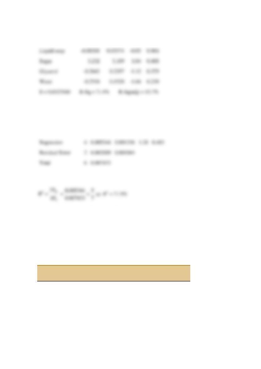
Regression
0.005344
0.001336
1.28
0.483
Residual Error
0.002089
0.001044
Total
0.007433
Reserve Supplemental Exercises Chapter 12 Problem 5
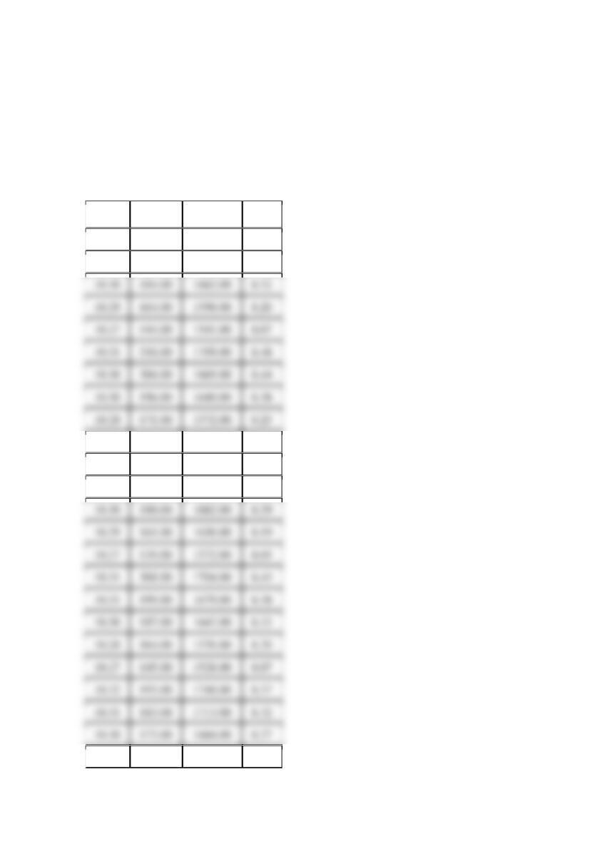
The data shown in the table below represent the thrust of a jet-turbine engine (y) and six
candidate regressors:
1
x
= primary speed of rotation,
2
x
= secondary speed of rotation,
3
x
= fuel
flow rate,
4
x
= pressure,
5
x
= exhaust temperature, and
6
x
= ambient temperature at time of test.
Fit the model using
*lnyy
=
as the response variable and
*
33
lnxx=
as the regressor (along with
4
x
and
5
x
).
Observation
Number
y
1
x
2
x
3
x
4
x
5
x
6
x
1
3540
2140
20640
30250
205
1732
99
2
4315
2016
20280
30010
195
1697
100
3
4095
1905
19860
29780
184
1662
97
4
4650
1675
18980
29330
164
1598
97
5
4200
1474
18100
28960
144
1541
97
6
4833
2239
20740
30083
216
1709
87
Liquid soap
-0.00268
-0.05
0.966
Sugar
3.232
1.04
0.408
Glycerol
0.2357
-1.12
0.379
Water
0.1520
-1.66
0.239
S = 0.0323160 R-Sq = 71.9% R-Sq(adj) = 15.7%
7
5617
2120
20305
29831
206
1669
87
8
4340
1990
19961
29604
196
1640
87
9
3820
1702
18916
29088
171
1572
85
10
3368
1487
18012
28675
149
1522
85
11
4445
2107
20520
30120
195
1740
101
12
4188
1973
20130
29920
190
1711
100
13
3981
1864
19780
29720
180
1682
100
14
3622
1674
19020
29370
161
1630
100
15
3125
1440
18030
28940
139
1572
101
16
4560
2165
20680
30160
208
1704
98
17
4340
2048
20340
29960
199
1679
96
18
4115
1916
19860
29710
187
1642
94
19
3630
1658
18950
29250
164
1576
94
20
3210
1489
18700
28890
145
1528
94
21
4330
2062
20500
30190
193
1748
101
22
4119
1929
20050
29960
183
1713
100
23
3891
1815
19680
29770
173
1684
100
24
3467
1595
18890
29360
153
1624
99
25
3045
1400
17870
28960
134
1569
100
26
4411
2047
20540
30160
193
1746
99
27
4203
1935
20160
29940
184
1714
99
28
3968
1807
19750
29760
173
1679
99
29
3531
1591
18890
29350
153
1621
99
30
3074
1388
17870
28910
133
1561
99
31
4350
2071
20460
30180
198
1729
102
32
4128
1944
20010
29940
186
1692
101
33
3940
1831
19640
29750
178
1667
101
34
3480
1612
18710
29360
156
1609
101
35
3064
1410
17780
28900
136
1552
101
36
4402
2066
20520
30170
197
1758
100
37
4180
1954
20150
29950
188
1729
99
38
3973
1835
19750
29740
178
1690
99
39
3530
1616
18850
29320
156
1616
99
40
3080
1407
17910
28910
137
1569
100
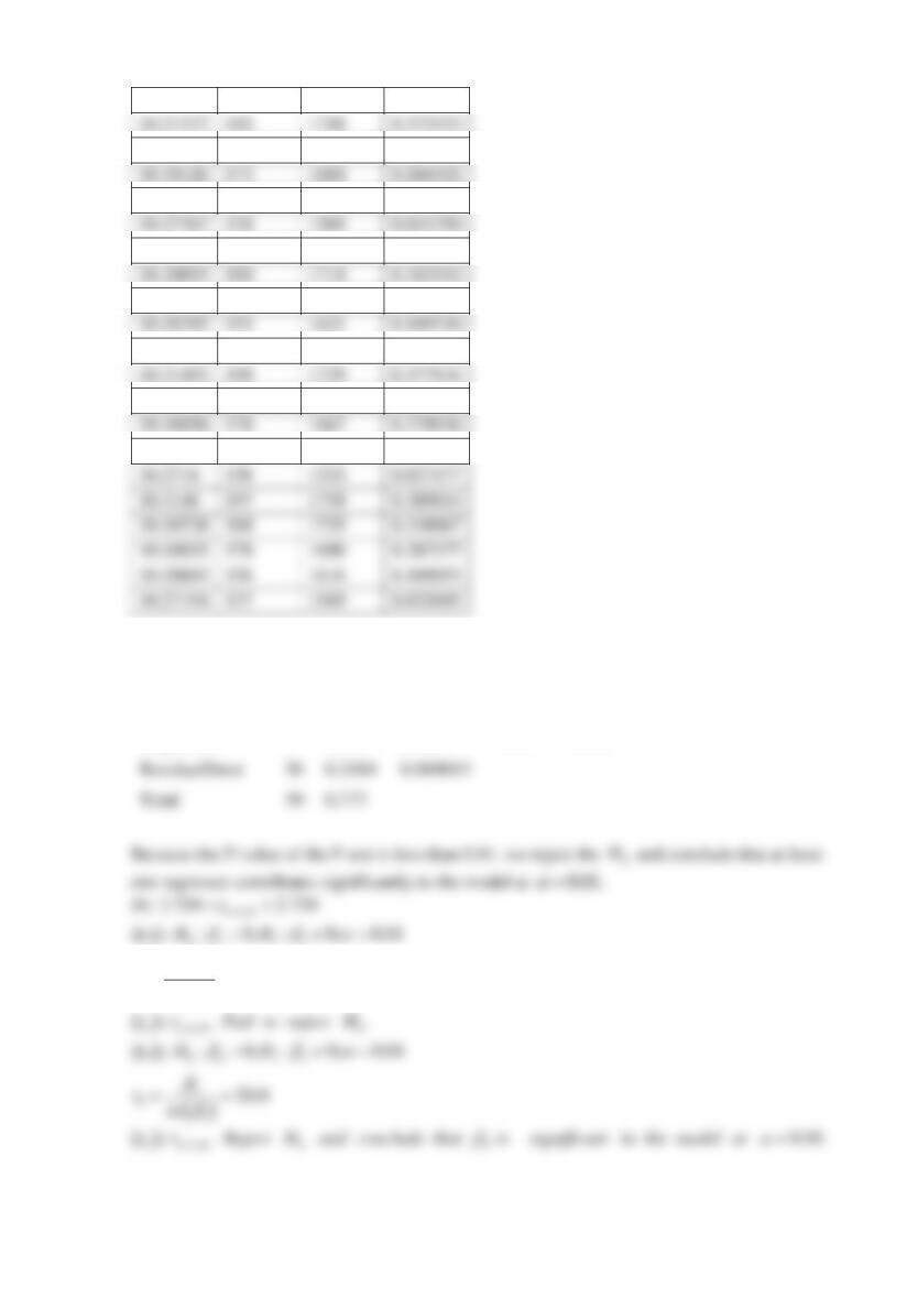
(a) Test for significance of regression using
0.01
=
. Find the P-value for this test and state your
conclusions.
(b) Use the t-statistic to test
0
H
:
0
j
=
versus
1
H
:
0
j
for each variable in the model. If
0.01
=
, what conclusions can you draw?
SOLUTION
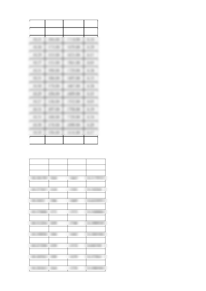
(a)
3
ln x
4
x
5
x
ln y
10.32
205.00
1732.00
8.42
10.31
195.00
1697.00
8.37
10.26
149.00
1522.00
8.12
10.31
195.00
1740.00
8.40
10.31
190.00
1711.00
8.34
10.30
180.00
1682.00
8.29
10.29
161.00
1630.00
8.19
10.27
139.00
1572.00
8.05
10.31
208.00
1704.00
8.43
10.31
199.00
1679.00
8.38
10.30
187.00
1642.00
8.32
10.28
164.00
1576.00
8.20
10.27
145.00
1528.00
8.07
10.32
193.00
1748.00
8.37
10.31
183.00
1713.00
8.32
10.30
173.00
1684.00
8.27
10.29
153.00
1624.00
8.15
10.30
184.00
1662.00
8.32
10.29
164.00
1598.00
8.20
10.27
144.00
1541.00
8.07
10.31
216.00
1709.00
8.48
10.30
206.00
1669.00
8.44
10.30
196.00
1640.00
8.38
10.28
171.00
1572.00
8.25
10.27
134.00
1569.00
8.02
10.31
193.00
1746.00
8.39
10.27
137.00
1569.00
8.03
10.31725
205
1732
8.171882
10.30929
195
1697
8.369853
10.30159
184
1662
8.317522
10.28637
164
1598
8.444622
10.27367
144
1541
8.34284
10.31172
216
1709
8.483223
10.3033
206
1669
8.633553
10.29566
196
1640
8.37563
10.27808
171
1572
8.248006
10.26378
149
1522
8.122074
10.31294
195
1740
8.399535
10.30628
190
1711
8.339979
10.29958
180
1682
8.289288
10.28773
161
1630
8.194782
10.27298
139
1572
8.04719
10.31427
208
1704
8.425078
10.29924
187
1642
8.322394
10.28363
164
1576
8.196988
10.31
184.00
1714.00
8.34
10.30
173.00
1679.00
8.29
10.29
153.00
1621.00
8.17
10.27
133.00
1561.00
8.03
10.31
198.00
1729.00
8.38
10.31
186.00
1692.00
8.33
10.30
178.00
1667.00
8.28
10.29
156.00
1609.00
8.15
10.27
136.00
1552.00
8.03
10.31
197.00
1758.00
8.39
10.31
188.00
1729.00
8.34
10.30
178.00
1690.00
8.29
10.29
156.00
1616.00
8.17
10.27125
145
1528
8.074026
10.30762
183
1713
8.323366
10.30126
173
1684
8.266421
10.28739
153
1624
8.151045
10.27367
134
1569
8.021256
10.31427
193
1746
8.391857
10.30695
184
1714
8.343554
10.30092
173
1679
8.286017
10.28705
153
1621
8.169336
10.27194
133
1561
8.030735
10.31493
198
1729
8.377931
10.30695
186
1692
8.325548
10.30058
178
1667
8.278936
10.28739
156
1609
8.154788
10.2716
136
1552
8.027477
10.3146
197
1758
8.389814
10.30728
188
1729
8.338067
10.30025
178
1690
8.287277
10.28603
156
1616
8.169053
10.27194
137
1569
8.032685
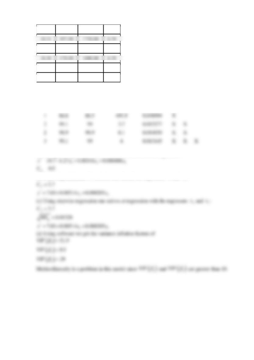
Analysis of Variance
Source
DF
SS
MS
F
P
Regression
3
0.559
0.186
30.71.
0.000
ResidualError
36
0.2184
0.000013
Total
39
0.777
0 3 1 3
( )
1
0
1
1.3tse
= = −
10.31527
193
1748
8.373323
Reserve Supplemental Exercises Chapter 12 Problem 6
The data shown in the table below represent the thrust of a jet-turbine engine (y) and six
candidate regressors:
1
x
= primary speed of rotation,
2
x
= secondary speed of rotation,
3
x
= fuel
flow rate,
4
x
= pressure,
5
x
= exhaust temperature, and
6
x
= ambient temperature at time of test.
Fit the model using
*lnyy
=
as the response variable and
*
33
lnxx=
as the regressor (along with
4
x
and
5
x
).
Observation
Number
y
1
x
2
x
3
x
4
x
5
x
6
x
1
4540
2140
20640
30250
205
1732
99
2
4315
2016
20280
30010
195
1697
100
3
4095
1905
19860
29780
184
1662
97
4
3650
1675
18980
29330
164
1598
97
5
3200
1474
18100
28960
144
1541
97
6
4833
2239
20740
30083
216
1709
87
7
4617
2120
20305
29831
206
1669
87
8
4340
1990
19961
29604
196
1640
87
9
3820
1702
18916
29088
171
1572
85
10
3368
1487
18012
28675
149
1522
85
11
4445
2107
20520
30120
195
1740
101
12
4188
1973
20130
29920
190
1711
100
13
3981
1864
19780
29720
180
1682
100
14
3622
1674
19020
29370
161
1630
100
15
3125
1440
18030
28940
139
1572
101
16
4560
2165
20680
30160
208
1704
98
17
4340
2048
20340
29960
199
1679
96
18
4115
1916
19860
29710
187
1642
94
19
3630
1658
18950
29250
164
1576
94
20
3210
1489
18700
28890
145
1528
94
21
4330
2062
20500
30190
193
1748
101
22
4119
1929
20050
29960
183
1713
100

23
3891
1815
19680
29770
173
1684
100
24
3467
1595
18890
29360
153
1624
99
25
3045
1400
17870
28960
134
1569
100
26
4411
2047
20540
30160
193
1746
99
27
4203
1935
20160
29940
184
1714
99
28
3968
1807
19750
29760
173
1679
99
29
3531
1591
18890
29350
153
1621
99
30
3074
1388
17870
28910
133
1561
99
31
4350
2071
20460
30180
198
1729
102
32
4128
1944
20010
29940
186
1692
101
33
3940
1831
19640
29750
178
1667
101
34
3480
1612
18710
29360
156
1609
101
35
3064
1410
17780
28900
136
1552
101
36
4402
2066
20520
30170
197
1758
100
37
4180
1954
20150
29950
188
1729
99
38
3973
1835
19750
29740
178
1690
99
39
3530
1616
18850
29320
156
1616
99
40
3080
1407
17910
28910
137
1569
100
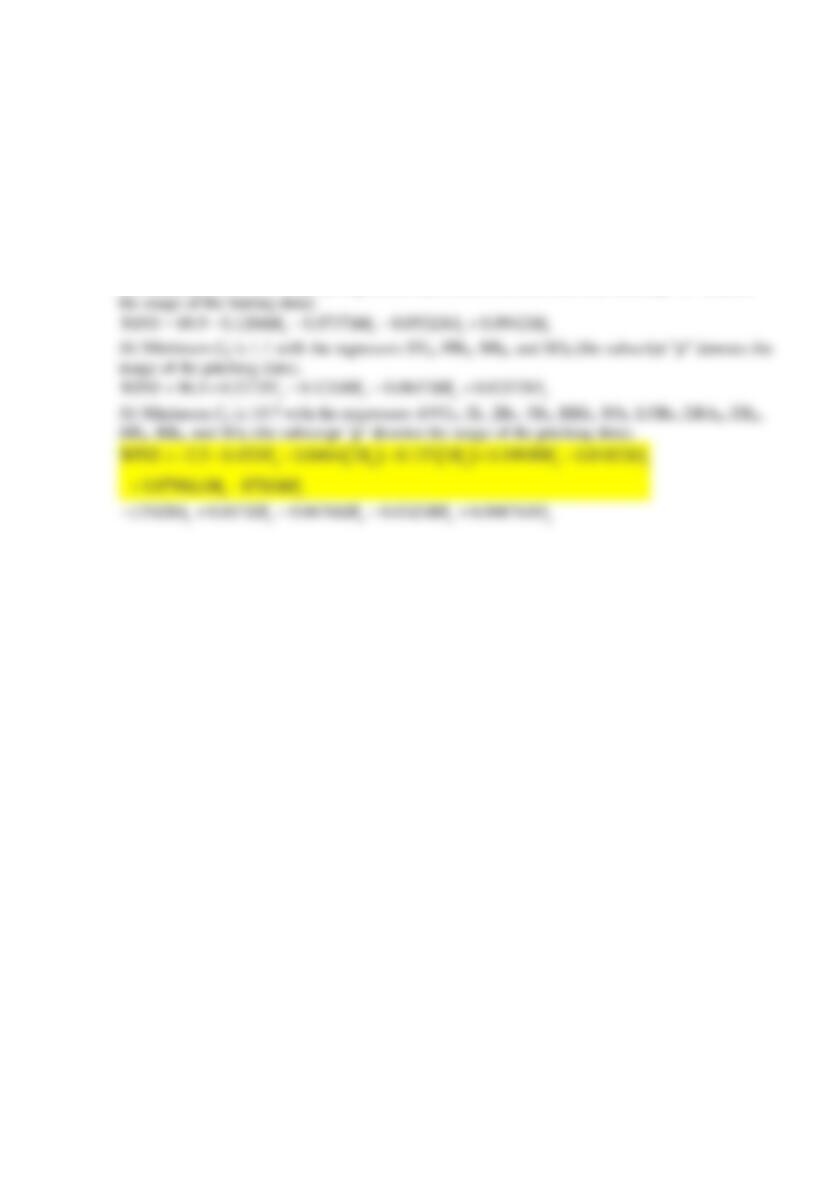
(a) Use all possible regressions to select the best regression equation, where the model with the
minimum value of MSE is to be selected as “best”.
(b) Repeat part (a) using the minimum
p
C
criterion to identify the best equation.
(c) Use stepwise regression to select a subset regression model.
(d) Compare the models obtained in parts (a), (b), and (c).
(e) Consider the three-variable regression model. Calculate the variance inflation factors for this
model.
Would you conclude that multicollinearity is a problem in this model?
SOLUTION
(a)
3
ln x
4
x
5
x
ln y
10.32
205.00
1732.00
8.42
10.31
195.00
1697.00
8.37
10.30
184.00
1662.00
8.32
10.27
144.00
1541.00
8.07
10.31
216.00
1709.00
8.48
10.30
206.00
1669.00
8.44
10.30
196.00
1640.00
8.38
10.28
171.00
1572.00
8.25
10.26
149.00
1522.00
8.12
10.31
195.00
1740.00
8.40
10.31
190.00
1711.00
8.34
10.30
180.00
1682.00
8.29
10.29
161.00
1630.00
8.19
10.27
139.00
1572.00
8.05
10.31
208.00
1704.00
8.43
10.31
199.00
1679.00
8.38
10.30
187.00
1642.00
8.32
10.28
164.00
1576.00
8.20
10.27
145.00
1528.00
8.07
10.32
193.00
1748.00
8.37
10.31
183.00
1713.00
8.32
10.30
173.00
1684.00
8.27
10.29
153.00
1624.00
8.15
10.27
134.00
1569.00
8.02
10.31
193.00
1746.00
8.39
10.31
184.00
1714.00
8.34
10.30
173.00
1679.00
8.29
10.29
153.00
1621.00
8.17
10.27
133.00
1561.00
8.03
10.31
198.00
1729.00
8.38
10.31
186.00
1692.00
8.33
10.29
164.00
1598.00
8.20
10.27
136.00
1552.00
8.03
10.31
188.00
1729.00
8.34
10.30
178.00
1690.00
8.29
10.29
156.00
1616.00
8.17
10.27
137.00
1569.00
8.03
Vars
R-Sq
R-Sq(adj)
Mallows
Cp
S
x3
x4
x5
1
98.8
98.7
14.1
0.015088
X
1
86.8
86.5
0.048994
X
2
99.1
0.013277
X
X
2
98.9
98.9
0.014030
X
X
3
99.1
0.013145
X
X
X
Following minimum MSE criterion one should use all three regressors:
(b) Following minimum CP criterion one should use regressors
4
x
and
5
x
:
Reserve Supplemental Exercises Chapter 12 Problem 7
Tables given below present statistics for the Major League Baseball season.
10.31
197.00
1758.00
8.39

Major League Baseball Season
American League Batting
Team
W
AVG
R
H
2B
3B
HR
RBI
BB
SO
SB
GIDP
LOB
OBP
Chicago
84
0.262
741
1450
253
23
200
713
435
1002
137
122
1032
0.322
Boston
95
0.281
910
1579
339
21
199
863
653
1044
45
135
1249
0.357
LA Angels
95
0.27
761
1520
278
30
147
726
447
848
161
125
1086
0.325
New York
95
0.276
886
1552
259
16
229
847
637
989
84
125
1264
0.355
Cleveland
93
0.271
790
1522
337
30
207
760
503
1093
62
128
1148
0.334
Oakland
88
0.262
772
1476
310
20
155
739
537
819
31
148
1170
0.33
Minnesota
83
0.259
688
1441
269
32
134
644
485
978
102
155
1109
0.323
Toronto
80
0.265
775
1480
307
39
136
735
486
955
72
126
1118
0.331
Texas
79
0.267
865
1528
311
29
260
834
495
1112
67
123
1104
0.329
Baltimore
59
0.269
729
1492
296
27
189
700
447
902
83
145
1103
0.327
Detroit
71
0.272
723
1521
283
45
168
678
384
1038
66
137
1077
0.321
Seattle
69
0.256
699
1408
289
34
130
657
466
986
102
115
1076
0.317
Tampa Bay
67
0.274
750
1519
289
40
157
717
412
990
151
133
1065
0.329
Kansas City
56
0.263
701
1445
289
34
126
653
424
1008
53
139
1062
0.32
National League Batting
Team
W
AVG
R
H
2B
3B
HR
RBI
BB
SO
SB
GIDP
LOB
OBP
St. Louis
100
0.27
805
1494
287
26
170
757
534
947
83
127
1152
0.339
Atlanta
90
0.265
769
1453
308
37
184
733
534
1084
92
146
1114
0.333

Houston
74
0.256
693
1400
281
32
161
654
481
1037
115
116
1136
0.322
Philadelphia
88
0.27
807
1494
282
35
167
760
639
1083
116
107
1251
0.348
Florida
83
0.272
717
1499
306
32
128
678
512
918
96
144
1181
0.339
New York
83
0.258
722
1421
279
32
175
683
486
1075
153
103
1122
0.322
San Diego
82
0.257
684
1416
269
39
130
655
600
977
99
122
1220
0.333
Milwaukee
81
0.259
726
1413
327
19
175
689
531
1162
79
137
1120
0.331
Washington
66
0.252
639
1367
311
32
117
615
491
1090
45
130
1137
0.322
Chicago
79
0.27
703
1506
323
23
194
674
419
920
65
131
1133
0.324
Arizona
77
0.256
696
1419
291
27
191
670
606
1094
67
132
1247
0.332
San Francisco
75
0.261
649
1427
299
26
128
617
431
901
71
147
1093
0.319
Cincinnati
73
0.261
820
1453
335
15
222
784
611
1303
72
116
1176
0.339
Los Angeles
71
0.253
685
1374
284
21
149
653
541
1094
58
139
1135
0.326
Colorado
67
0.267
740
1477
280
34
150
704
509
1103
65
125
1197
0.333
Pittsburgh
82
0.259
680
1445
292
38
139
656
471
1092
73
130
1193
0.322
Major League Baseball 2005
American League Pitching
Team
W
ERA
SV
H
R
ER
HR
BB
SO
AVG
Chicago
84
3.61
54
1392
645
592
167
459
1040
0.249
Boston
95
4.74
38
1550
805
752
164
440
959
0.276
LA Angels
95
3.68
54
1419
643
598
158
443
1126
0.254

New York
95
4.52
46
1495
789
718
164
463
985
0.269
Cleveland
93
3.61
51
1363
642
582
157
413
1050
0.247
Oakland
88
3.69
38
1315
658
594
154
504
1075
0.241
Minnesota
83
3.71
44
1458
662
604
169
348
965
0.261
Toronto
80
4.06
35
1475
705
653
185
444
958
0.264
Texas
79
4.96
46
1589
858
794
159
522
932
0.279
Baltimore
59
4.56
38
1458
800
724
180
580
1052
0.263
Detroit
71
4.51
37
1504
787
719
193
461
907
0.272
Seattle
69
4.49
39
1483
751
712
179
496
892
0.268
Tampa Bay
67
5.39
43
1570
936
851
194
615
949
0.28
Kansas City
56
5.49
25
1640
935
862
178
580
924
0.291
National League Pitching
Team
W
ERA
SV
H
R
ER
HR
BB
SO
AVG
St. Louis
100
3.49
48
1399
634
560
153
443
974
0.257
Atlanta
90
3.98
38
1487
674
639
145
520
929
0.268
Houston
74
3.51
45
1336
609
563
155
440
1164
0.246
Philadelphia
88
4.21
40
1379
726
672
189
487
1159
0.253
Florida
83
4.16
42
1459
732
666
116
563
1125
0.266
New York
83
3.76
38
1390
648
599
135
491
1012
0.255
San Diego
82
4.13
45
1452
726
668
146
503
1133
0.259
Milwaukee
81
3.97
46
1382
697
635
169
569
1173
0.251
Washington
66
3.87
51
1456
673
627
140
539
997
0.262
Chicago
79
4.19
39
1357
714
671
186
576
1256
0.25
Arizona
77
4.84
45
1580
856
783
193
537
1038
0.278
San Francisco
75
4.33
46
1456
745
695
151
592
972
0.263
Cincinnati
73
5.15
31
1657
889
820
219
492
955
0.29
Los Angeles
71
4.38
40
1434
755
695
182
471
1004
0.263
Colorado
67
5.13
37
1600
862
808
175
604
981
0.287
Pittsburgh
82
4.42
35
1456
769
706
162
612
958
0.267
Batting
LOB
Left on base
W
Wins
OBP
On-base percentage
AVG
Batting average
R
Runs
Pitching
H
Hits
ERA
Earned run average
2B
Doubles
SV
Saves
3B
Triples
H
Hits
HR
Home runs
R
Runs
RBI
Runs batted in
ER
Earned runs
BB
Walks
HR
Home runs
SO
Strikeouts
BB
Walks
SB
Stolen bases
SO
Strikeouts
GIDP
Grounded into double play
AVG
Opponent batting average
(a) Consider the batting data. Use model-building methods to predict wins from the other
variables. Use Cp criterion.
(b) Repeat part (a) for the pitching data.
(c) Use both the batting and pitching data to build a model to predict wins.
SOLUTION
(a) Minimum Cp is –1.3 with the regressors HRb, BBb, SOb, and SBb (the subscript “b” denotes