Applied Statistics and Probability for Engineers, 7th edition 2017
CHAPTER 12
Sections 12.1
12.1.1 Exercise 11.2.1. described a regression model between percent of body fat (%BF) as measured by immersion and BMI
from a study on 250 male subjects. The researchers also measured 13 physical characteristics of each man, including
his age (yrs), height (in), and waist size (in.).
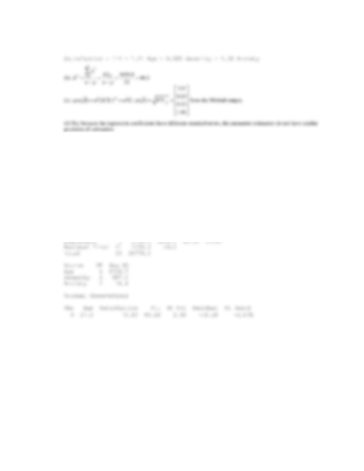
A regression of percent of body fat with both height and waist as predictors shows the following computer output:
Estimate Std. Error t-value Pr (>|t|)
(Intercept) −3.10088 7.68611 −0.403 0.687
Height −0.60154 0.10994 −5.472 1.09e−07
Waist 1.77309 0.07158 24.770 <2e−16
Residual standard error: 4.46 on 247 degrees of freedom
Multiple R-squared: 0.7132, Adjusted R-squared: 0.7109
F-statistic: 307.1 on 2 and 247 DF, p-value: <2.2e−16
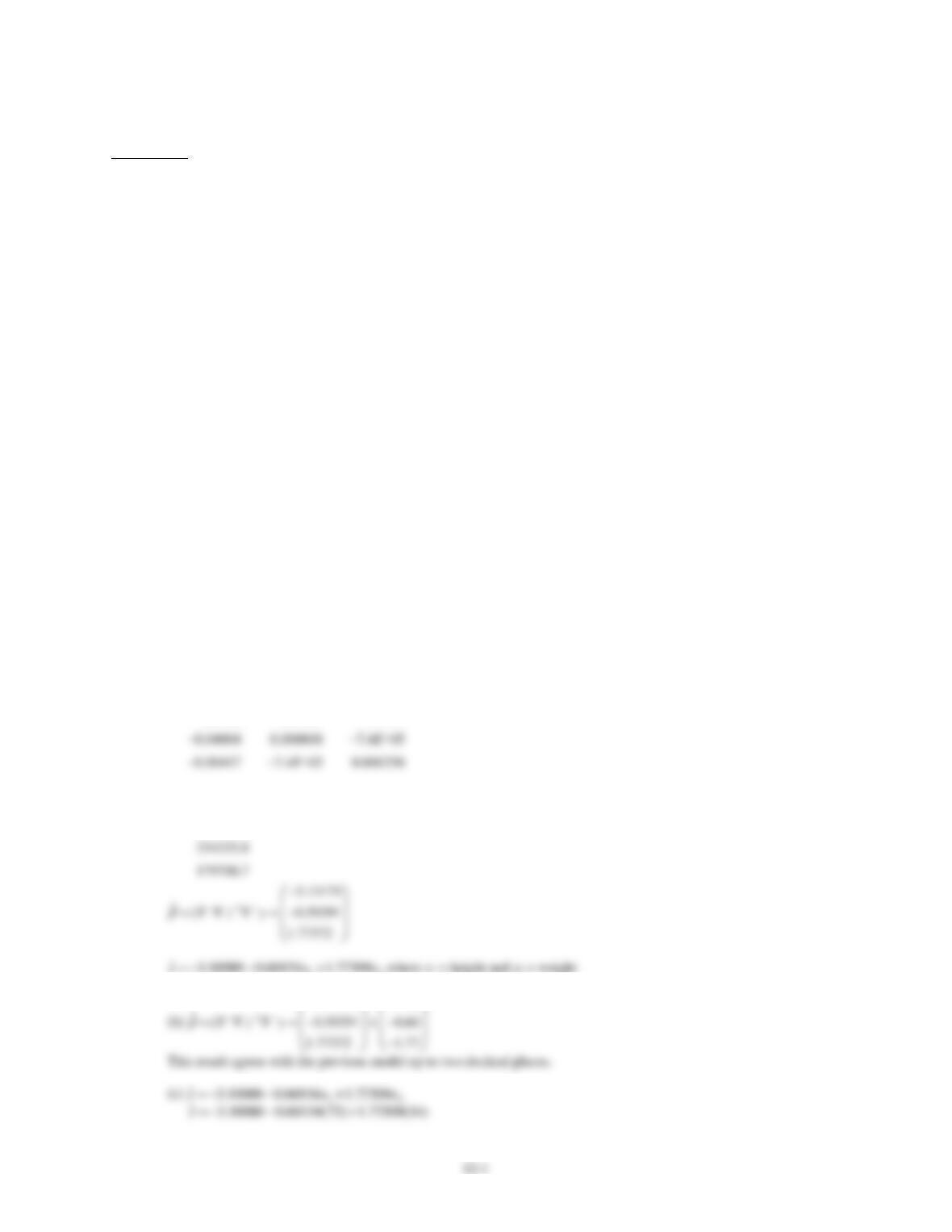
(a) Write out the regression model if
−
− − − −
= − − − −
− − − −
1
2.9705 4.0042 2 4.1679 2
( ) 0.04004 6.0774 4 7.3875 5
0.00417 7.3875 5 2.5766 4
EE
EE
EE
XX
and
( )
4757.9
= 334335.8
179706.7
Xy
(b) Verify that the model found from technology is correct to at least 2 decimal places.
(c) What is the predicted body fat of a man who is 6-ft tall with a 34-in waist?
(a)
(XX)−1 =
Xy =
12
−
−
3.13171 3.10
2.9705
−0.04004
−0.0417
4757.9
12-2
=
ˆ13.87y
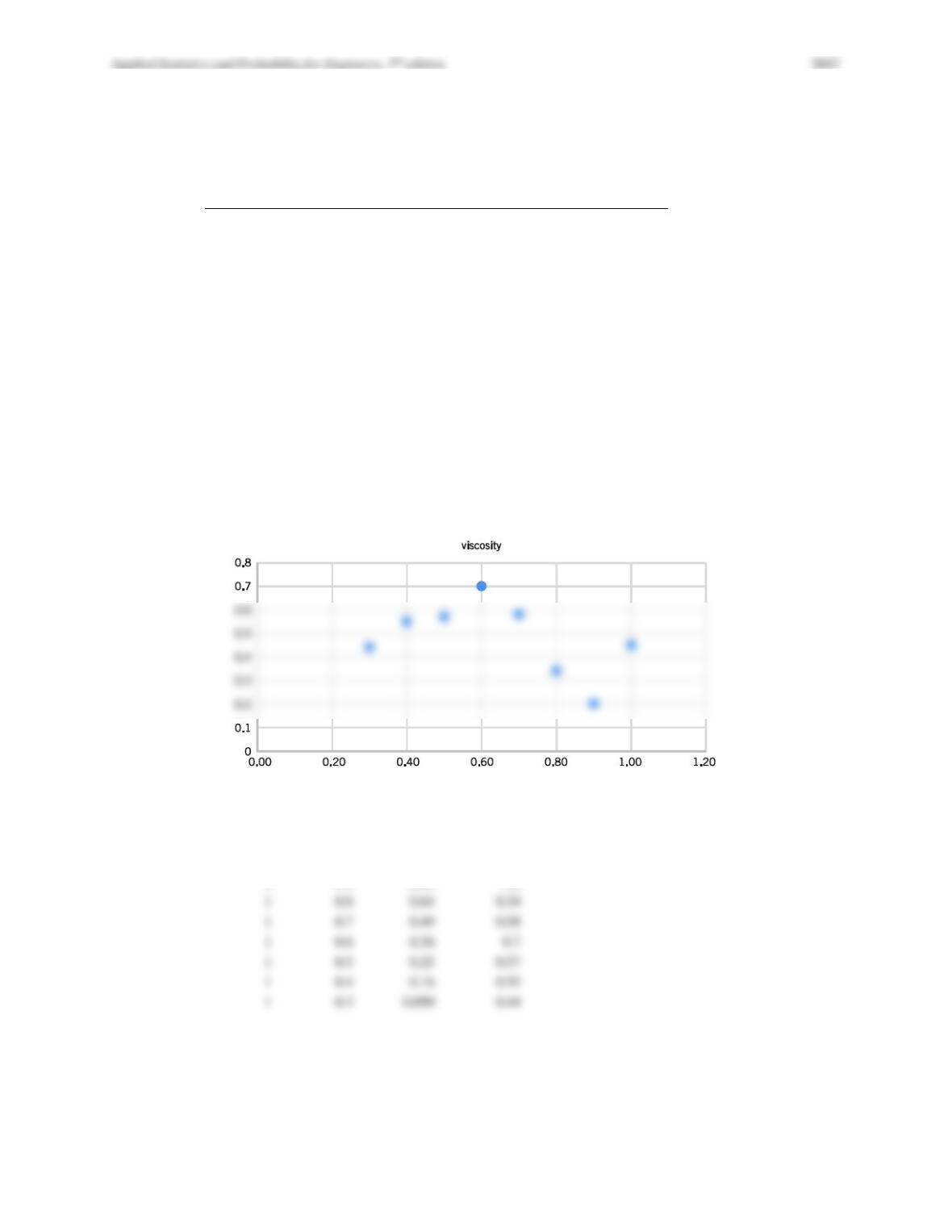
12.1.2 Hsuie, Ma, and Tsai (‘‘Separation and Characterizations of Thermotropic Copolyesters of p-Hydroxybenzoic Acid,
Sebacic Acid, and Hydroquinone,’’ (1995, Vol. 56) studied the effect of the molar ratio of sebacic acid (the regressor)
on the intrinsic viscosity of copolyesters (the response). The following display presents the data.
Ratio
Viscosity
1.0
0.45
0.9
0.20
0.8
0.34
0.7
0.58
0.6
0.70
0.5
0.57
0.4
0.55
0.3
0.44
(a) Construct a scatterplot of the data.
(b) Fit a second-order prediction equation.
(a)
(b) To fit a second order model, the ratio term is squared
1
0.8
0.64
1
0.7
0.49
1
0.6
0.36
0.7
1
0.5
0.25
1
0.4
0.16
1
0.3
0.090
Intercept
Ratio
Ratio2
Viscosity
1.00
1.00
1.00
0.450
1
0.9
0.81
0.2
Applied Statistics and Probability for Engineers, 7th edition 2017
12-3
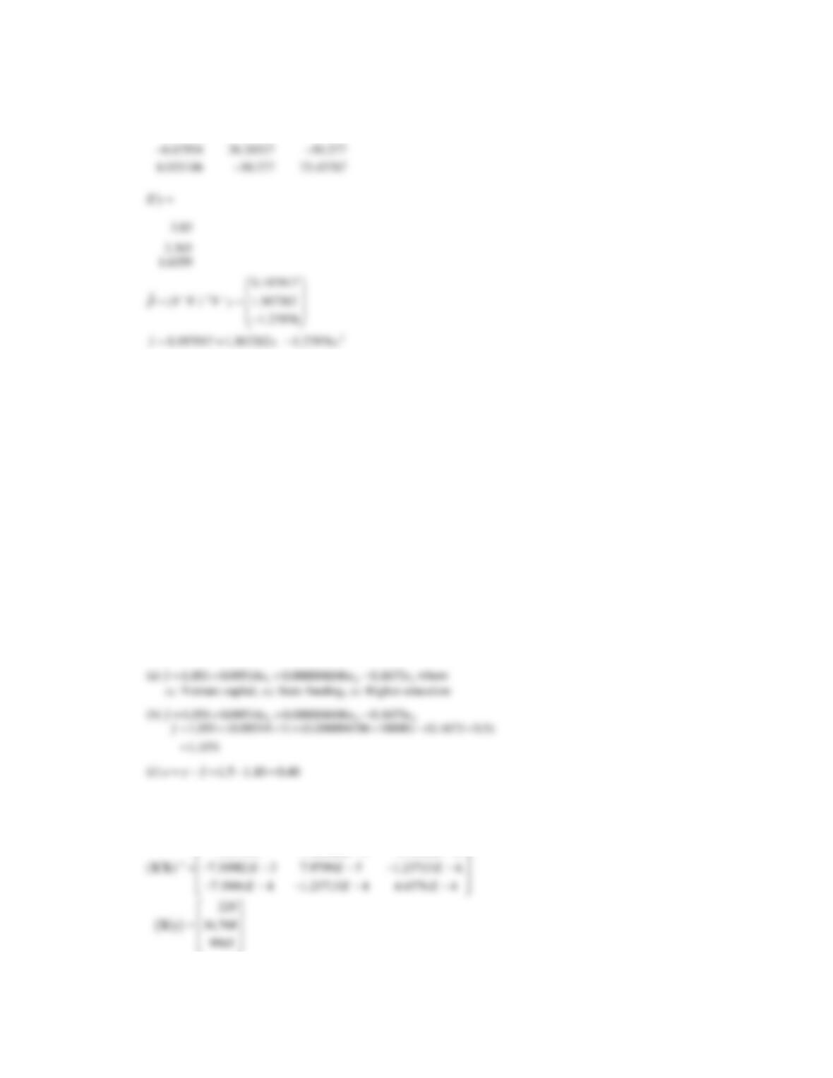
(XʹX)−1 =
12.1.3 Can the percentage of the workforce who are engineers in each U.S. state be predicted by the amount of money spent in
on higher education (as a percent of gross domestic product), on venture capital (dollars per $1000 of gross domestic
product) for high-tech business ideas, and state funding (in dollars per student) for major research universities? Data for
all 50 states and a software package revealed the following results:
Estimate
Std. Error
t value
Pr (>|t|)
(Intercept)
1.051e+00
1.567e−01
6.708
2.5e−08***
Venture cap
9.514e−02
3.910e−02
2.433
0.0189*
State funding
4.106e−06
1.437e−05
0.286
0.7763
Higher Ed
−
1.673e−01
2.595e−01
−
0.645
0.5223
Residual standard error: 0.3007 on 46 degrees of freedom
Multiple R-squared: 0.1622, Adjusted R-squared: 0.1075
F-statistic: 2.968 on 3 and 46 DF, p-value: 0.04157
(a) Write the equation predicting the percent of engineers in the workforce.
(b) For a state that has $1 per $1000 in venture capital, spends $10,000 per student on funding for major research
universities, and spends 0.5% of its GDP on higher education, what percent of engineers do you expect to see in the
workforce?
(c) If the state in part (b) actually had 1.5% engineers in the workforce, what would the residual be?
12.1.4 A regression model is to be developed for predicting the ability of soil to absorb chemical contaminants. Ten
observations have been taken on a soil absorption index (y) and two regressors: x1 = amount of extractable iron ore and
x2 = amount of bauxite. We wish to fit the model y =
0 +
1x1 +
2x2 + ϵ. Some necessary quantities are
− − − −
1.17991 7.30982 3 7.3006 4
EE
1.872356
−
6.67954
8.055106
6.67954
36.28527
50.277
Applied Statistics and Probability for Engineers, 7th edition 2017
12-4
(a) Estimate the regression coefficients in the model specified.
(b) What is the predicted value of the absorption index y when x1 = 200 and x2 = 50?
12.1.5 The data from a patient satisfaction survey in a hospital are shown next.
Observation
Age
Severity
Surg-Med
Anxiety
Satisfaction
1
55
50
0
2.1
68
2
46
24
1
2.8
77
3
30
46
1
3.3
96
4
35
48
1
4.5
80
5
59
58
0
2.0
43
6
61
60
0
5.1
44
7
74
65
1
5.5
26
8
38
42
1
3.2
88
9
27
42
0
3.1
75
10
51
50
1
2.4
57
11
53
38
1
2.2
56
12
41
30
0
2.1
88
13
37
31
0
1.9
88
14
24
34
0
3.1
102
15
42
30
0
3.0
88
16
50
48
1
4.2
70
17
58
61
1
4.6
52
18
60
71
1
5.3
43
19
62
62
0
7.2
46
20
68
38
0
7.8
56
21
70
41
1
7.0
59
22
79
66
1
6.2
26
23
63
31
1
4.1
52
24
39
42
0
3.5
83
25
49
40
1
2.1
75
The regressor variables are the patient’s age, an illness severity index (higher values indicate greater severity), an
indicator variable denoting whether the patient is a medical patient (0) or a surgical patient (1), and an anxiety index
(higher values indicate greater anxiety).
(a) Fit a multiple linear regression model to the satisfaction response using age, illness severity, and the anxiety index
as the regressors.
(b) Estimate
2.
(c) Find the standard errors of the regression coefficients.
(d) Are all of the model parameters estimated with nearly the same precision? Why or why not?
Applied Statistics and Probability for Engineers, 7th edition 2017
12-5
(a) The results from computer software follow. The model can be expressed as
REGRESSION ANALYSIS: SATISFACTION VERSUS AGE, SEVERITY, ANXIETY
The regression equation is
Satisfaction = 144 − 1.11 Age − 0.585 Severity + 1.30 Anxiety
Predictor Coef SE Coef T P
Constant 143.895 5.898 24.40 0.000
Age −1.1135 0.1326 −8.40 0.000
Severity −0.5849 0.1320 −4.43 0.000
Anxiety 1.296 1.056 1.23 0.233
S = 7.03710 R-Sq = 90.4% R-Sq(adj) = 89.0%
Analysis of Variance
Source DF SS MS F P
12.1.6 The electric power consumed each month by a chemical plant is thought to be related to the average ambient
temperature (x1), the number of days in the month (x2), the average product purity (x3), and the tons of product
produced (x4). The past year’s historical data are available and are presented below.
(a) Fit a multiple linear regression model to these data.
(b) Estimate
2.
(c) Compute the standard errors of the regression coefficients.
Are all of the model parameters estimated with the same precision? Why or why not?
Applied Statistics and Probability for Engineers, 7th edition 2017
12-6
(d) Predict power consumption for a month in which x1 = 75°F, x2 = 24 days, x3 = 90%, and x4 = 98 tons.
y
x1
x2
x3
x4
240
25
24
91
100
236
31
21
90
95
270
45
24
88
110
274
60
25
87
88
301
65
25
91
94
316
72
26
94
99
300
80
25
87
97
296
84
25
86
96
267
75
24
88
110
276
60
25
91
105
288
50
25
90
100
261
38
23
89
98
Predictor Coef SE Coef T P
Constant −123.1 157.3 −0.78 0.459
X1 0.7573 0.2791 2.71 0.030
X2 7.519 4.010 1.87 0.103
X3 2.483 1.809 1.37 0.212
X4 −0.4811 0.5552 −0.87 0.415
S = 11.79 R-Sq = 85.2% R-Sq(adj) = 76.8%
Analysis of Variance
Source DF SS MS F P
Regression 4 5600.5 1400.1 10.08 0.005
Residual Error 7 972.5 138.9
Total 11 6572.9
Applied Statistics and Probability for Engineers, 7th edition 2017
12-7
12.1.7 An article in Electronic Packaging and Production (2002, Vol. 42) considered the effect of X-ray inspection of
integrated circuits. The rads (radiation dose) were studied as a function of current (in milliamps) and exposure time (in
minutes). The data are shown below.
Rads
mAmps
Exposure Time
7.4
10
0.25
14.8
10
0.5
29.6
10
1
59.2
10
2
88.8
10
3
296
10
10
444
10
15
592
10
20
11.1
15
0.25
22.2
15
0.5
44.4
15
1
88.8
15
2
133.2
15
3
444
15
10
666
15
15
888
15
20
14.8
20
0.25
29.6
20
0.5
59.2
20
1
118.4
20
2
177.6
20
3
592
20
10
888
20
15
1184
20
20
22.2
30
0.25
44.4
30
0.5
88.8
30
1
177.6
30
2
266.4
30
3
888
30
10
1332
30
15
1776
30
20
29.6
40
0.25
59.2
40
0.5
118.4
40
1
236.8
40
2
355.2
40
3
1184
40
10
1776
40
15
2368
40
20
(a) Fit a multiple linear regression model to these data with rads as the response.
(b) Estimate
2
and the standard errors of the regression coefficients.
Applied Statistics and Probability for Engineers, 7th edition 2017
12-8
(c) Use the model to predict rads when the current is 15 milliamps and the exposure time is 5 seconds.
The regression equation is
rads = − 440 + 19.1 mAmps + 68.1 exposure time
Predictor Coef SE Coef T P
Constant −440.39 94.20 −4.68 0.000
mAmps 19.147 3.460 5.53 0.000
exposure time 68.080 5.241 12.99 0.000
S = 235.718 R-Sq = 84.3% R-Sq(adj) = 83.5%
Analysis of Variance
Source DF SS MS F P
Regression 2 11076473 5538237 99.67 0.000
Residual Error 37 2055837 55563
Total 39 13132310
12.1.8 The pull strength of a wire bond is an important characteristic. The table below gives information on pull strength (y),
die height (x1), post height (x2), loop height (x3), wire length (x4), bond width on the die (x5), and bond width on the post
(x6).
(a) Fit a multiple linear regression model using x2, x3, x4, and x5 as the regressors.
(b) Estimate
2.
(c) Find the
ˆ
( ).
j
se
How precisely are the regression coefficients estimated in your opinion?
(d) Use the model from part (a) to predict pull strength when x2 = 20, x3 = 30, x4 = 90, and x5 = 2.0.
y
x1
x2
x3
x4
x5
x6
8.0
5.2
19.6
29.6
94.9
2.1
2.3
8.3
5.2
19.8
32.4
89.7
2.1
1.8
8.5
5.8
19.6
31.0
96.2
2.0
2.0
8.8
6.4
19.4
32.4
95.6
2.2
2.1
9.0
5.8
18.6
28.6
86.5
2.0
1.8
9.3
5.2
18.8
30.6
84.5
2.1
2.1
9.3
5.6
20.4
32.4
88.8
2.2
1.9
9.5
6.0
19.0
32.6
85.7
2.1
1.9
9.8
5.2
20.8
32.2
93.6
2.3
2.1
10.0
5.8
19.9
31.8
86.0
2.1
1.8
10.3
6.4
18.0
32.6
87.1
2.0
1.6
10.5
6.0
20.6
33.4
93.1
2.1
2.1
10.8
6.2
20.2
31.8
83.4
2.2
2.1
11.0
6.2
20.2
32.4
94.5
2.1
1.9
11.3
6.2
19.2
31.4
83.4
1.9
1.8
11.5
5.6
17.0
33.2
85.2
2.1
2.1
11.8
6.0
19.8
35.4
84.1
2.0
1.8
12.3
5.8
18.8
34.0
86.9
2.1
1.8
12.5
5.6
18.6
34.2
83.0
1.9
2.0
Applied Statistics and Probability for Engineers, 7th edition 2017
12-9
The regression equation is
y = 7.46 − 0.030 x2 + 0.521 x3 − 0.102 x4 − 2.16 x5
Predictor Coef StDev T P
Constant 7.458 7.226 1.03 0.320
x2 −0.0297 0.2633 −0.11 0.912
x3 0.5205 0.1359 3.83 0.002
x4 −0.10180 0.05339 −1.91 0.077
x5 −2.161 2.395 −0.90 0.382
S = 0.8827 R-Sq = 67.2% R-Sq(adj) = 57.8%
Analysis of Variance
Source DF SS MS F P
Regression 4 22.3119 5.5780 7.16 0.002
Error 14 10.9091 0.7792
Total 18 33.2211
12.1.9 An article in IEEE Transactions on Instrumentation and Measurement (2001, Vol. 50, pp. 2033–2040) reported on
a study that had analyzed powdered mixtures of coal and limestone for permittivity. The errors in the density
measurement were the response. The data are reported in the following table.
Density
Dielectric Constant
Loss Factor
0.749
2.05
0.016
0.798
2.15
0.02
0.849
2.25
0.022
0.877
2.3
0.023
0.929
2.4
0.026
0.963
2.47
0.028
0.997
2.54
0.031
1.046
2.64
0.034
1.133
2.85
0.039
1.17
2.94
0.042
1.215
3.05
0.045
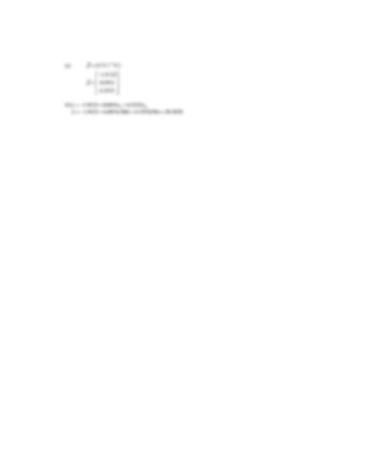
(a) Fit a multiple linear regression model to these data with the density as the response.
(b) Estimate
2
and the standard errors of the regression coefficients.
(c) Use the model to predict the density when the dielectric constant is 2.5 and the loss factor is 0.03.
The regression equation is
density = − 0.110 + 0.407 dielectric constant + 2.11 loss factor
Predictor Coef SE Coef T P
Constant −0.1105 0.2501 −0.44 0.670
dielectric constant 0.4072 0.1682 2.42 0.042
loss factor 2.108 5.834 0.36 0.727
S = 0.00883422 R-Sq = 99.7% R-Sq(adj) = 99.7%
Analysis of Variance
Source DF SS MS F P
Regression 2 0.23563 0.11782 1509.64 0.000
Residual Error 8 0.00062 0.00008
Applied Statistics and Probability for Engineers, 7th edition 2017
12-10
Total 10 0.23626
12.1.10 An article in Biotechnology Progress (2001, Vol. 17, pp. 366–368) reported on an experiment to investigate and
optimize nisin extraction in aqueous two-phase systems (ATPS). The nisin recovery was the dependent variable (y).
The two regressor variables were concentration (%) of PEG 4000 (denoted as x1 and concentration (%) of Na2SO4
(denoted as x2). The data are in the table below.
x1
x2
y
13
11
62.8739
15
11
76.1328
13
13
87.4667
15
13
102.3236
14
12
76.1872
14
12
77.5287
14
12
76.7824
14
12
77.4381
14
12
78.7417
(a) Fit a multiple linear regression model to these data.
(b) Estimate
2
and the standard errors of the regression coefficients.
(c) Use the model to predict the nisin recovery when x1 = 14.5 and x2 = 12.5.
The regression equation is
y = − 171 + 7.03 x1 + 12.7 x2
Predictor Coef SE Coef T P
Constant −171.26 28.40 −6.03 0.001
x1 7.029 1.539 4.57 0.004
x2 12.696 1.539 8.25 0.000
S = 3.07827 R-Sq = 93.7% R-Sq(adj) = 91.6%
Analysis of Variance
Source DF SS MS F P
Regression 2 842.37 421.18 44.45 0.000
Residual Error 6 56.85 9.48
Total 8 899.22
12.1.11 An article in Optical Engineering [“Operating Curve Extraction of a Correlator’s Filter” (2004, Vol. 43, pp. 2775–
2779)] reported on the use of an optical correlator to perform an experiment by varying brightness and contrast. The
resulting modulation is characterized by the useful range of gray levels. The data follow
Brightness (%): 54 61 65 100 100 100 50 57 54
Contrast (%): 56 80 70 50 65 80 25 35 26
Applied Statistics and Probability for Engineers, 7th edition 2017
Useful range (ng): 96 50 50 112 96 80 155 144 255
(a) Fit a multiple linear regression model to these data.
(b) Estimate
2.
(c) Compute the standard errors of the regression coefficients.
(d) Predict the useful range when brightness = 80 and contrast = 75.
The regression equation is
Useful range (ng) = 239 + 0.334 Brightness (%) − 2.72 Contrast (%)
Predictor Coef SE Coef T P
Constant 238.56 45.23 5.27 0.002
Brightness (%) 0.3339 0.6763 0.49 0.639
Contrast (%) −2.7167 0.6887 −3.94 0.008
S = 36.3493 R-Sq = 75.6% R-Sq(adj) = 67.4%
Analysis of Variance
Source DF SS MS F P
Regression 2 24518 12259 9.28 0.015
Residual Error 6 7928 1321
Total 8 32446

12-12
12.1.12 Regression Analysis: W versus GF, GA, …
The table below presents statistics for the National Hockey League teams from the 2008–2009 season (The Sports
Network). Fit a multiple linear regression model that relates wins to the variables GF through F. Because teams play 82
game, W = 82 − L
−
T − OTL, but such a model does not help build a better team. Estimate
2
and find the standard
errors of the regression coefficients for your model.
Team
W
L
OTL
PTS
GF
GA
ADV
PPGF
PCTG
PEN
BMI
AVG
SHT
PPGA
PKPCT
SHGF
SHGA
FG
Anaheim
42
33
7
91
238
235
309
73
23.6
1418
8
17.4
385
78
79.7
6
6
43
Atlanta
35
41
6
76
250
279
357
69
19.3
1244
12
15.3
366
88
76
13
9
39
Boston
53
19
10
116
270
190
313
74
23.6
1016
12
12.5
306
54
82.4
8
7
47
Buffalo
41
32
9
91
242
229
358
75
21
1105
16
13.7
336
61
81.8
7
4
44
Carolina
45
30
7
97
236
221
374
70
18.7
786
16
9.8
301
59
80.4
8
7
39
Columbus
41
31
10
92
220
223
322
41
12.7
1207
20
15
346
62
82.1
8
9
41
Calgary
46
30
6
98
251
246
358
61
17
1281
18
15.8
349
58
83.4
6
13
37
Chicago
46
24
12
104
260
209
363
70
19.3
1129
28
14.1
330
64
80.6
10
5
43
Colorado
32
45
5
69
190
253
318
50
15.7
1044
18
13
318
64
79.9
4
5
31
Dallas
36
35
11
83
224
251
351
54
15.4
1134
10
14
327
70
78.6
2
2
38
Detroit
51
21
10
112
289
240
353
90
25.5
810
14
10
327
71
78.3
6
4
46
Edmonton
38
35
9
85
228
244
354
60
17
1227
20
15.2
338
76
77.5
3
8
39
Florida
41
30
11
93
231
223
308
51
16.6
884
16
11
311
54
82.6
7
6
39
Los Angeles
34
37
11
79
202
226
360
69
19.2
1191
16
14.7
362
62
82.9
4
7
39
Minnesota
40
33
9
89
214
197
328
66
20.1
869
20
10.8
291
36
87.6
9
6
39
Montreal
41
30
11
93
242
240
374
72
19.2
1223
6
15
370
65
82.4
10
10
38
New Jersey
51
27
4
106
238
207
307
58
18.9
1038
20
12.9
324
65
79.9
12
3
44
Nashville
40
34
8
88
207
228
318
50
15.7
982
12
12.1
338
59
82.5
9
8
41
NY Islanders
26
47
9
61
198
274
320
54
16.9
1198
18
14.8
361
73
79.8
12
5
37
NY Rangers
43
30
9
95
200
212
346
48
13.9
1175
24
14.6
329
40
87.8
9
13
42
Ottawa
36
35
11
83
213
231
339
66
19.5
1084
14
13.4
346
64
81.5
8
5
46
Philadelphia
44
27
11
99
260
232
316
71
22.5
1408
26
17.5
393
67
83
16
1
43
Phoenix
36
39
7
79
205
249
344
50
14.5
1074
18
13.3
293
68
76.8
5
4
36
Pittsburgh
45
28
9
99
258
233
360
62
17.2
1106
8
13.6
347
60
82.7
7
11
46
San Jose
53
18
11
117
251
199
360
87
24.2
1037
16
12.8
306
51
83.3
12
10
46
St. Louis
41
31
10
92
227
227
351
72
20.5
1226
22
15.2
357
58
83.8
10
8
35
Tampa Bay
24
40
18
66
207
269
343
61
17.8
1280
26
15.9
405
89
78
4
8
34
Toronto
34
35
13
81
244
286
330
62
18.8
1113
12
13.7
308
78
74.7
6
7
40
Vancouver
45
27
10
100
243
213
357
67
18.8
1323
28
16.5
371
69
81.4
7
5
47
Washington
50
24
8
108
268
240
337
85
25.2
1021
20
12.7
387
75
80.6
7
9
45
W Wins
L Losses during regular time
OTL Overtime losses
PTS Points. Two points for winning a game, one point for a tie or losing in overtime, zero points for losing in regular
time.
GF Goals for
GA Goals against
ADV Total advantages. Power-play opportunities.
PPGF Power-play goals for. Goals scored while on power play.
PCTG Power-play percentage. Power-play goals divided by total advantages.
PEN Total penalty minutes including bench minutes
BMI Total bench minor minutes
AVG Average penalty minutes per game
SHT Total times short-handed. Measures opponent opportunities.
PPGA Power-play goals against
PKPCT Penalty killing percentage. Measures a team’s ability to prevent goals while its opponent is a power play. Opponent
opportunities minus power-play goals divided by opponent’s opportunities.
SHGF Short-handed goals for
SHGA Short-handed goals against
FG Games scored first
Applied Statistics and Probability for Engineers, 7th edition 2017
12-13
The regression equation is
W = 512 + 0.164 GF − 0.183 GA − 0.054 ADV + 0.09 PPGF − 0.14 PCTG − 0.163 PEN
− 0.128 BMI + 13.1 AVG + 0.292 SHT − 1.60 PPGA − 5.54 PKPCT + 0.106 SHGF
+ 0.612 SHGA + 0.005 FG
Predictor Coef SE Coef T P
Constant 512.2 185.9 2.75 0.015
GF 0.16374 0.03673 4.46 0.000
GA −0.18329 0.04787 −3.83 0.002
ADV −0.0540 0.2183 −0.25 0.808
PPGF 0.089 1.126 0.08 0.938
PCTG −0.142 3.810 −0.04 0.971
PEN −0.1632 0.3029 −0.54 0.598
BMI −0.1282 0.2838 −0.45 0.658
AVG 13.09 24.84 0.53 0.606
SHT 0.2924 0.1334 2.19 0.045
PPGA −1.6018 0.6407 −2.50 0.025
PKPCT −5.542 2.181 −2.54 0.023
SHGF 0.1057 0.1975 0.54 0.600
SHGA 0.6124 0.2615 2.34 0.033
FG 0.0047 0.1943 0.02 0.981
S = 2.65443 R-Sq = 92.9% R-Sq(adj) = 86.3%
Analysis of Variance
12.1.13 A study was performed on wear of a bearing and its relationship to x1 = oil viscosity and x2 = load. The following data
were obtained.
y
x1
x2
293
1.6
851
230
15.5
816
172
22.0
1058
91
43.0
1201
113
33.0
1357
125
40.0
1115
(a) Fit a multiple linear regression model to these data.
(b) Estimate
2 and the standard errors of the regression coefficients.
(c) Use the model to predict wear when x1 = 25 and x2 = 1000.
(d) Fit a multiple linear regression model with an interaction term to these data.
Applied Statistics and Probability for Engineers, 7th edition 2017
12-14
(e) Estimate
2 and
β
ˆ
()
j
se
for this new model. How did these quantities change? Does this tell you anything about the
value of adding the interaction term to the model?
(f) Use the model in part (d) to predict when x1 = 25 and x2 = 1000. Compare this prediction with the predicted value
from part (c).
Predictor Coef SE Coef T P
Constant 383.80 36.22 10.60 0.002
Xl −3.6381 0.5665 −6.42 0.008
X2 −0.11168 0.04338 −2.57 0.082
S = 12.35 R−Sq = 98.5% R−Sq(adj) = 97.5%
Analysis of Variance
Source DF SS MS F P
Regression 2 29787 14894 97.59 0.002
Residual Error 3 458 153
Total 5 30245
Sections 12-2
12.2.1 Recall the regression of percent of body fat on height and waist from Exercise 12.1.1. The simple regression model of
percent of body fat on height alone shows the following:
Estimate Std. Error t value Pr (>|t|)
(Intercept) 25.58078 14.15400 1.807 0.0719
Height −0.09316 0.20119 −0.463 0.6438
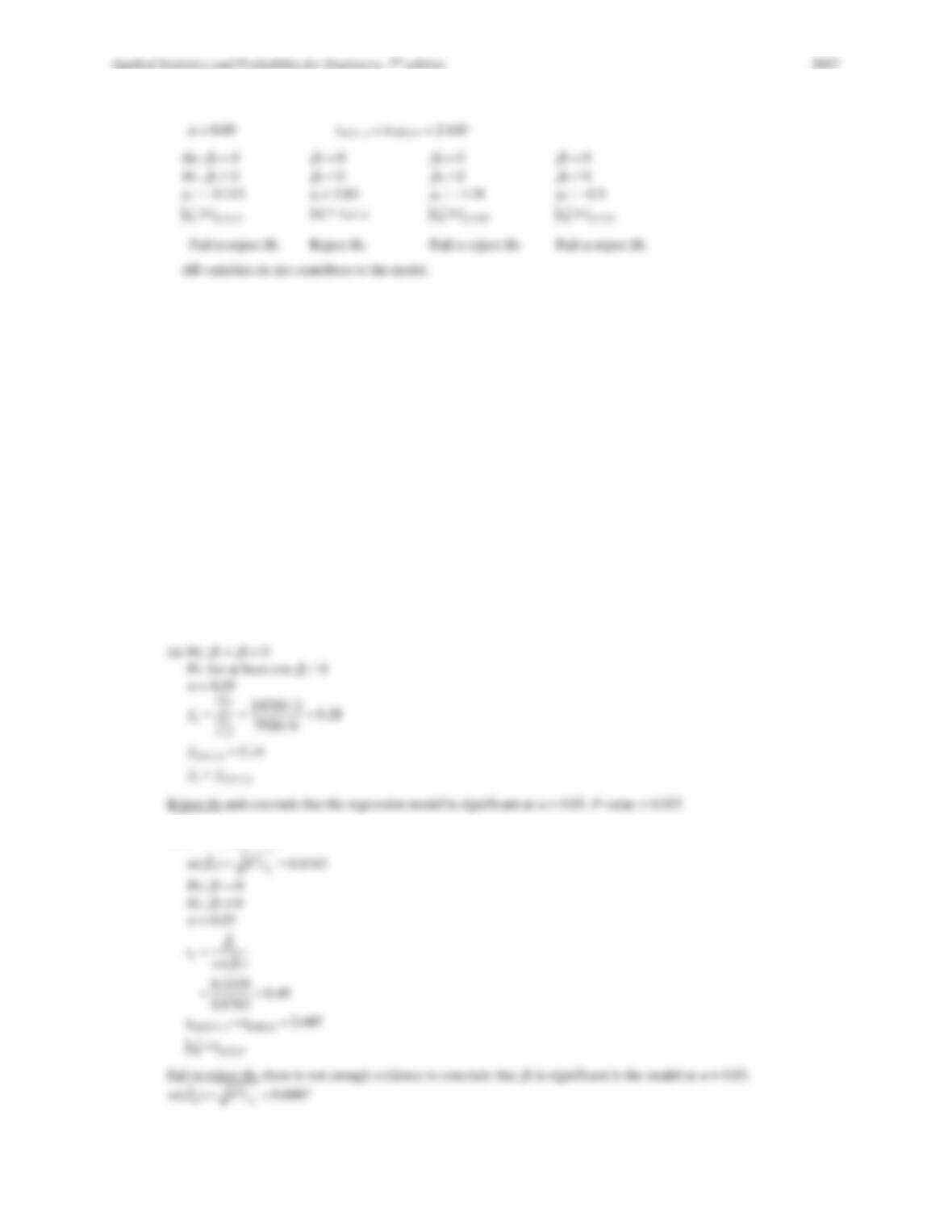
(a) Test whether the coefficient of height is statistically significant.
(b) Looking at the model with both waist and height in the model, test whether the coefficient of height is significant in
this model.
(c) Explain the discrepancy in your two answers.
Applied Statistics and Probability for Engineers, 7th edition 2017
12-15
12.2.2 Consider the linear regression model from Exercise 12.1.2. Is the second-order term necessary in the regression model?
Computer output for the model with ratio and ratio squared is shown below. The P-value for the test of whether the
coefficient of ratio squared equals zero is 0.309 > 0.05. Therefore, there is not sufficient evidence that the ratio
squared variable is useful to the model.
The regression equation is
viscosity = 0.198 + 1.37 ratio − 1.28 ratio2
Predictor Coef SE Coef T P
Constant 0.1979 0.4466 0.44 0.676
ratio 1.367 1.488 0.92 0.400
ratio2 −1.280 1.131 −1.13 0.309
S = 0.146606 R−Sq = 37.5% R−Sq(adj) = 12.5%
Analysis of Variance
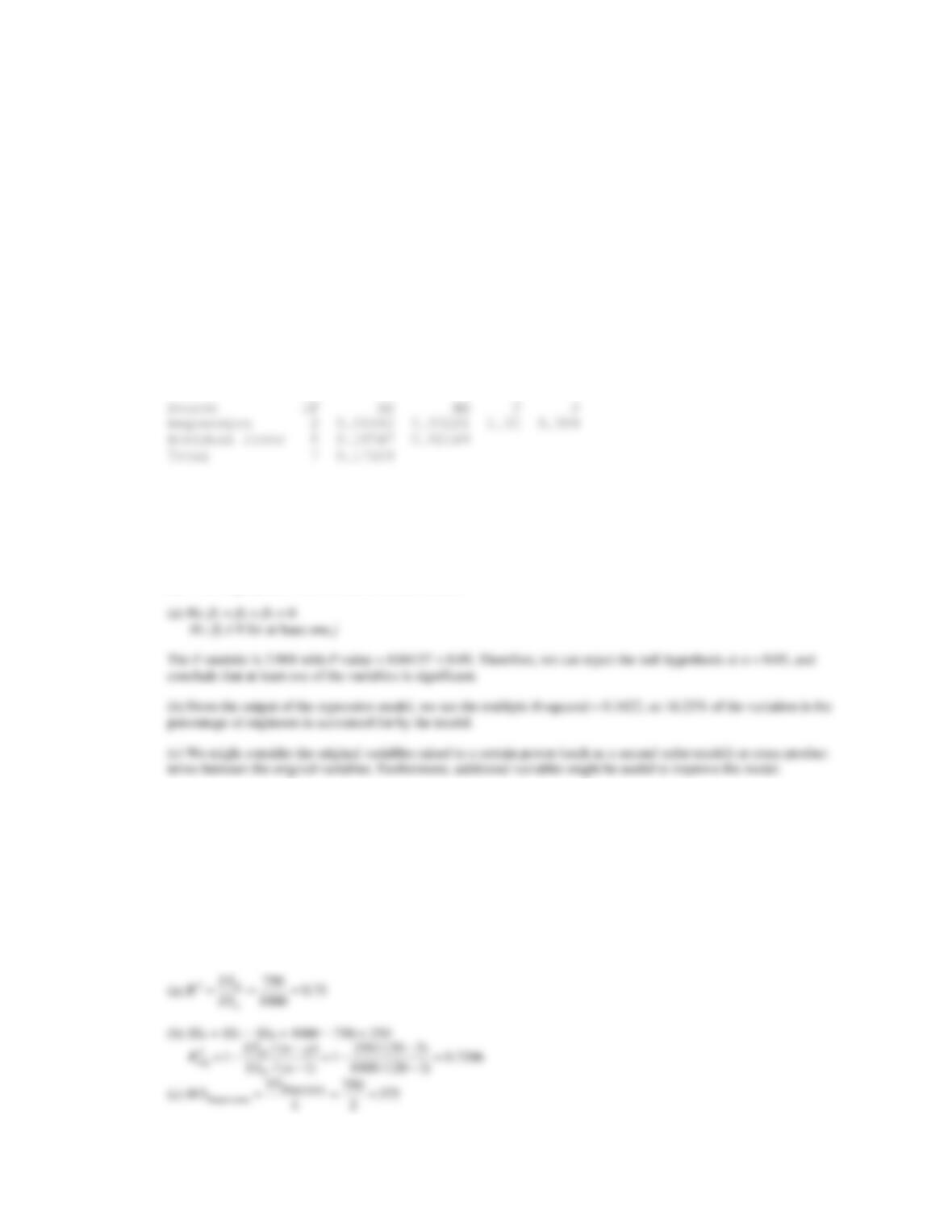
12.2.3 Consider the regression model of Exercise 12.1.3 attempting to predict the percent of engineers in the workforce from
various spending variables.
(a) Are any of the variables useful for prediction? (Test an appropriate hypothesis).
(b) What percent of the variation in the percent of engineers is accounted for by the model?
(c) What might you do next to create a better model?
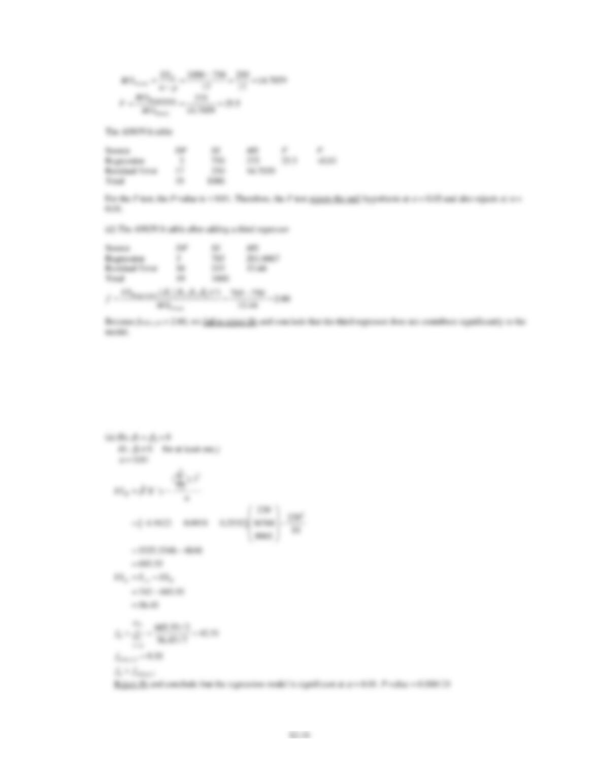
12.2.4 You have fit a regression model with two regressors to a data set that has 20 observations. The total sum of squares is
1000 and the model sum of squares is 750.
(a) What is the value of R2 for this model?
(b) What is the adjusted R2 for this model?
(c) What is the value of the F-statistic for testing the significance of regression? What conclusions would you draw
about this model if
= 0.05? What if
= 0.01?
(d) Suppose that you add a third regressor to the model and as a result, the model sum of squares is now 785. Does it
seem to you that adding this factor has improved the model?
Applied Statistics and Probability for Engineers, 7th edition 2017
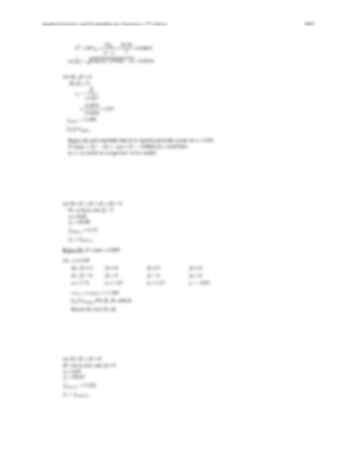
12.2.5 Consider the absorption index data in Exercise 12.1.4. The total sum of squares for y is SST = 742.00.
(a) Test for significance of regression using
= 0.01. What is the P-value for this test?
(b) Test the hypothesis H0:
1 = 0 versus H1:
1≠ 0 using
= 0.01. What is the P-value for this test?
(c) What conclusion can you draw about the usefulness of x1 as a regressor in this model?
Syy = 742.00
12-17
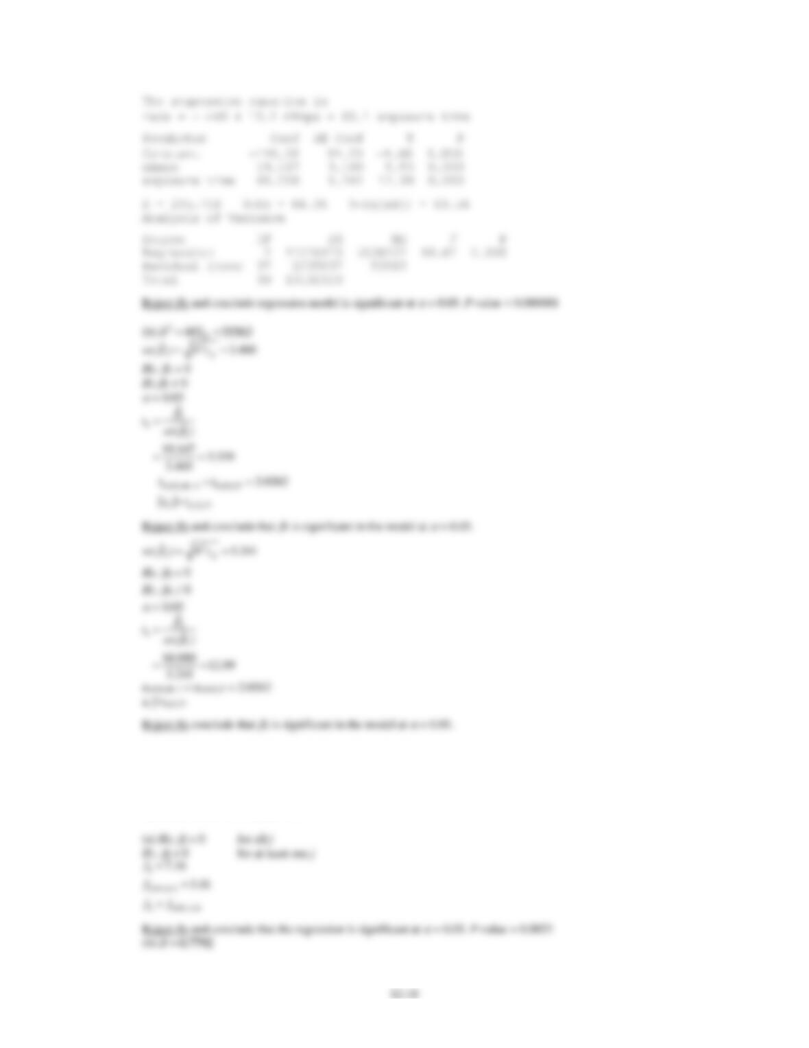
12.2.6 Consider the electric power consumption data in Exercise 12.1.6.
(a) Test for significance of regression using
= 0.05. What is the P-value for this test?
(b) Use the t-test to assess the contribution of each regressor to the model. Using
= 0.05, what conclusions can you
draw?
12.2.7 Consider the regression model fit to the X-ray inspection data in Exercise 12.1.7. Use rads as the response.
(a) Test for significance of regression using
= 0.05. What is the P-value for this test?
(b) Construct a t-test on each regression coefficient. What conclusions can you draw about the variables in this model?
Use
= 0.05.
Applied Statistics and Probability for Engineers, 7th edition 2017
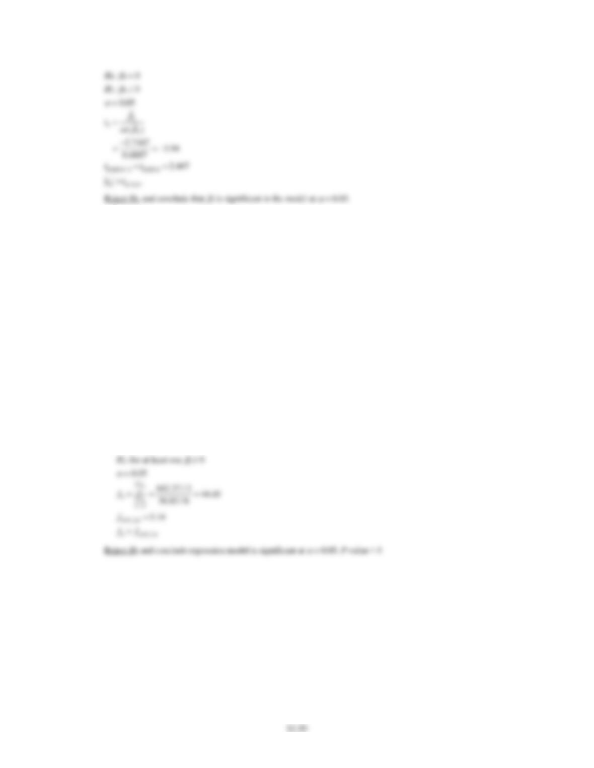
12.2.8 Consider the wire bond pull strength data in Exercise 12.1.8.
(a) Test for significance of regression using
= 0.05. Find the P-value for this test. What conclusions can you draw?
(b) Calculate the t-test statistic for each regression coefficient. Using
= 0.05, what conclusions can you draw? Do all
variables contribute to the model?
12-19
12.2.9 Consider the regression model fit to the gray range modulation data in Exercise 12.1.11. Use the useful range as the
response.
(a) Test for significance of regression using
= 0.05. What is the P-value for this test?
(b) Construct a t-test on each regression coefficient. What conclusions can you draw about the variables in this model?
Use
= 0.05.
Useful range (ng) = 239 + 0.334 Brightness (%) − 2.72 Contrast (%)
Predictor Coef SE Coef T P
Constant 238.56 45.23 5.27 0.002
Brightness (%) 0.3339 0.6763 0.49 0.639
Contrast (%) −2.7167 0.6887 −3.94 0.008
S = 36.3493 R−Sq = 75.6% R−Sq(adj) = 67.4%
Analysis of Variance
Source DF SS MS F P
Regression 2 24518 12259 9.28 0.015
Residual Error 6 7928 1321
Total 8 32446
(b)
==
2
ˆ1321
E
MS
Applied Statistics and Probability for Engineers, 7th edition 2017
12.2.10 Consider the regression model fit to the nisin extraction data in Exercise 12.1.10. Use nisin extraction as the response.
(a) Test for significance of regression using
= 0.05. What is the P-value for this test?
(b) Construct a t-test on each regression coefficient. What conclusions can you draw about the variables in this
model?
Use
= 0.05.
(c) Comment on the effect of a small sample size to the tests in the previous parts.
The regression equation is
y = − 171 + 7.03 x1 + 12.7 x2
Predictor Coef SE Coef T P
Constant −171.26 28.40 −6.03 0.001
x1 7.029 1.539 4.57 0.004
x2 12.696 1.539 8.25 0.000
S = 3.07827 R−Sq = 93.7% R−Sq(adj) = 91.6%
Analysis of Variance
Source DF SS MS F P
Regression 2 842.37 421.18 44.45 0.000
Residual Error 6 56.85 9.48
Total 8 899.22
(a) H0:
1 =
2 = 0