
Differential Equations
for Engineers:
the Essentials
Class 11 notes
Agenda: Class 11
Review Homework Assignment 9
Lectures:
Second order linear time-invariant nonhomogeneous ODEs
(1) Procedure and example for the kernel method
Homework Assignment 11

Second Order Linear Time-Invariant
Nonhomogeneous ODEs
Procedure and Example for Variation of
Parameters (Kernel) Method
Procedure for the Kernel Method
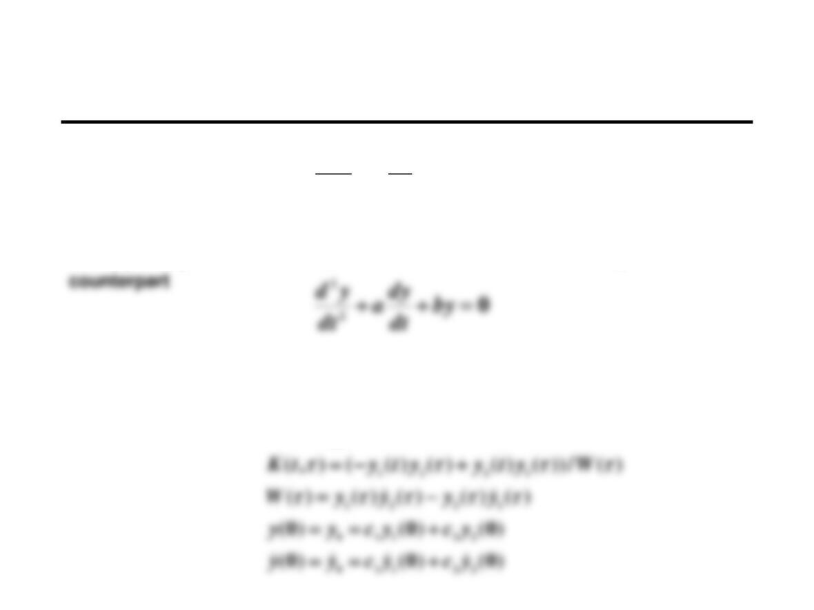
If the ODE to be solved is
and are fundamental solutions to the ODE’s homogeneous
then the formulae for the Kernel Method are:
)(),()(
)()()()(
0
2211
dgtKty
tyctyctyty
t
P
P
=
++=
)0(,)0(
)(
00
2
2
==
=++
yyyy
tgby
dt
dy
a
dt
yd
)(),(21 tyty
Equation 1
Procedure for the Kernel Method (2)
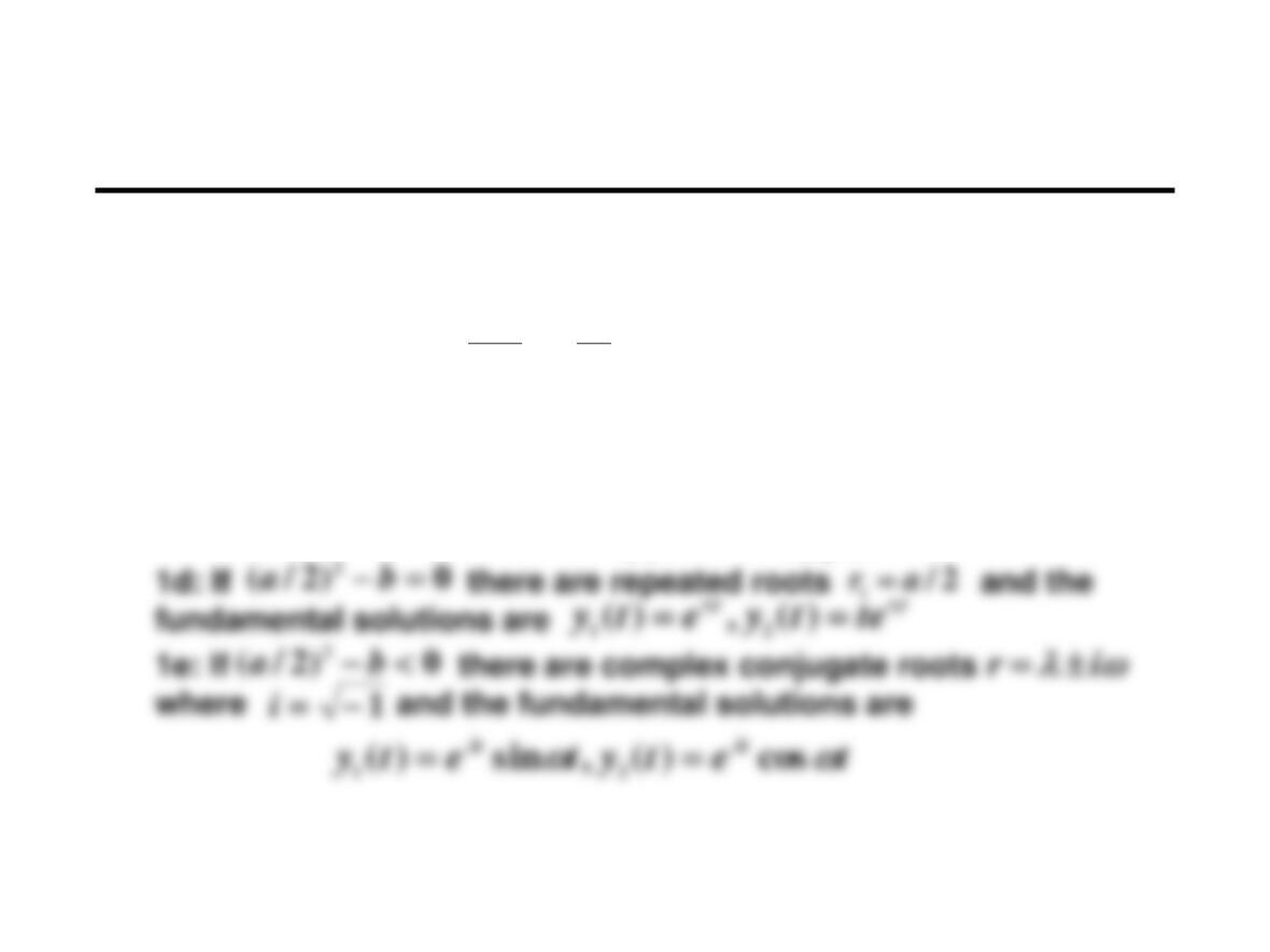
Step 1: Find the fundamental solutions to the homogeneous ODE:
1a: Try
1b: Solve the resulting characteristic equation
1c: If there are two distinct real roots and
the fundamental solutions are
0
2
2
=++ by
dt
dy
a
dt
yd
rt
ety =)(
0
2=++ barr
0)2/( 2− ba
21 ,rr
trtr etyety 21 )(,)( 21 ==
Procedure for the Kernel Method (3)
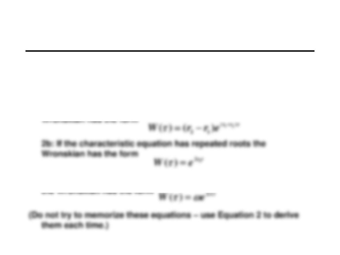
Step 2: Calculate the Wronskian
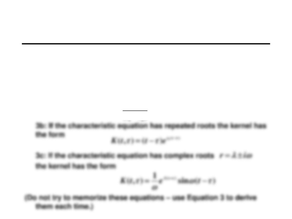
2a: If the characteristic equation has two distinct roots the
2c: If the characteristic equation has complex roots
)()()()()( 1221
yyyyW −=
ir =
Equation 2
Procedure for the Kernel Method (4)
Step 3: Calculate the kernel
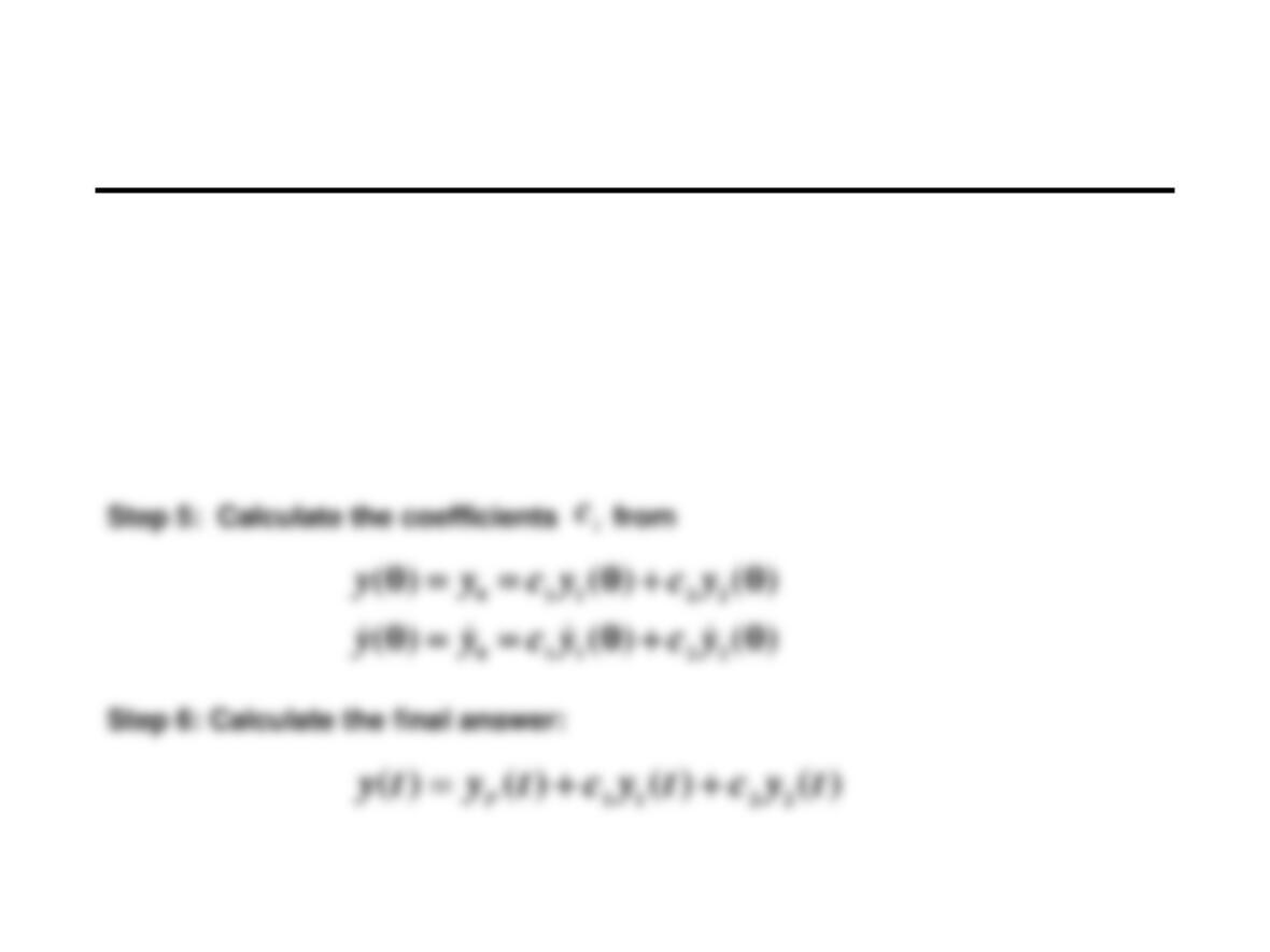
3a: If the characteristic equation has two distinct roots the kernel
has the form
)(/))()()()((),( 1221
WytyytytK +−=
Equation 3
)(
)(
1
),( )()(
21
−− −
−
=trtr ee
rr
tK
Procedure for the Kernel Method (5)
Step 4: Perform the integration to determine the particular solution:
For the three types of roots to the characteristic equation and for the common
kinds of input functions , the integrals will usually be one of the
forms listed on the next chart.
)(
g
=t
PdgtKty 0)(),()(
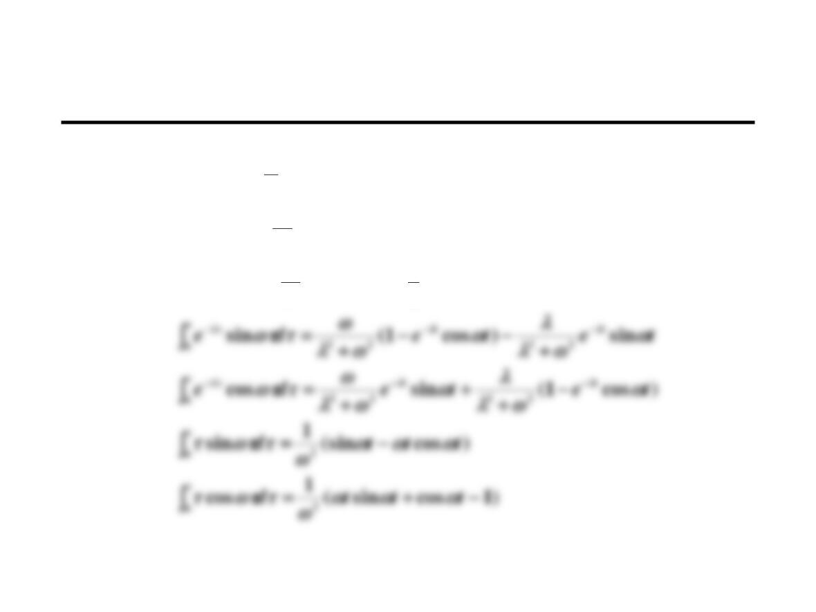
Table of Common Integrals
)))(
2
1
1(1(
2
))1(1(
1
)1(
1
2
3
0
2
02
0
++−=
+−=
−=
−−
−−
−−
ettde
etde
ede
t
t
tt
t
t
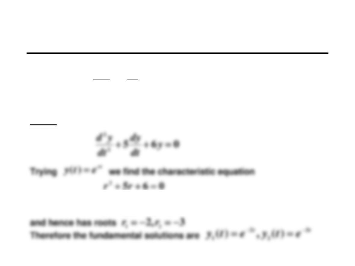
(Do not try to memorize these integrals –be able to derive them each time)
Kernel Method: Example
Solve:
Step 1: Find the fundamental solutions to
which factors into
1)0(
65
2
2
=
=++ −
y
ey
dt
dy
dt
yd t
0)3)(2( =++ rr
1)0( −=
y
Kernel Method: Example (2)
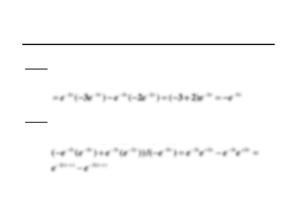
Step 2: Calculate the Wronskian
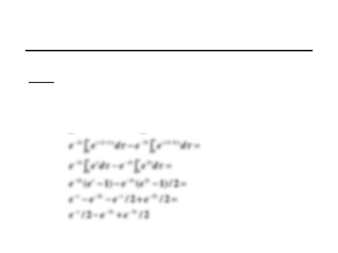
Step 3: Calculate the kernel
1221
)()()()()(
−=
yyyyW
1221
)(/))()()()((),(
=+−=
WytyytytK
Kernel Method: Example (3)
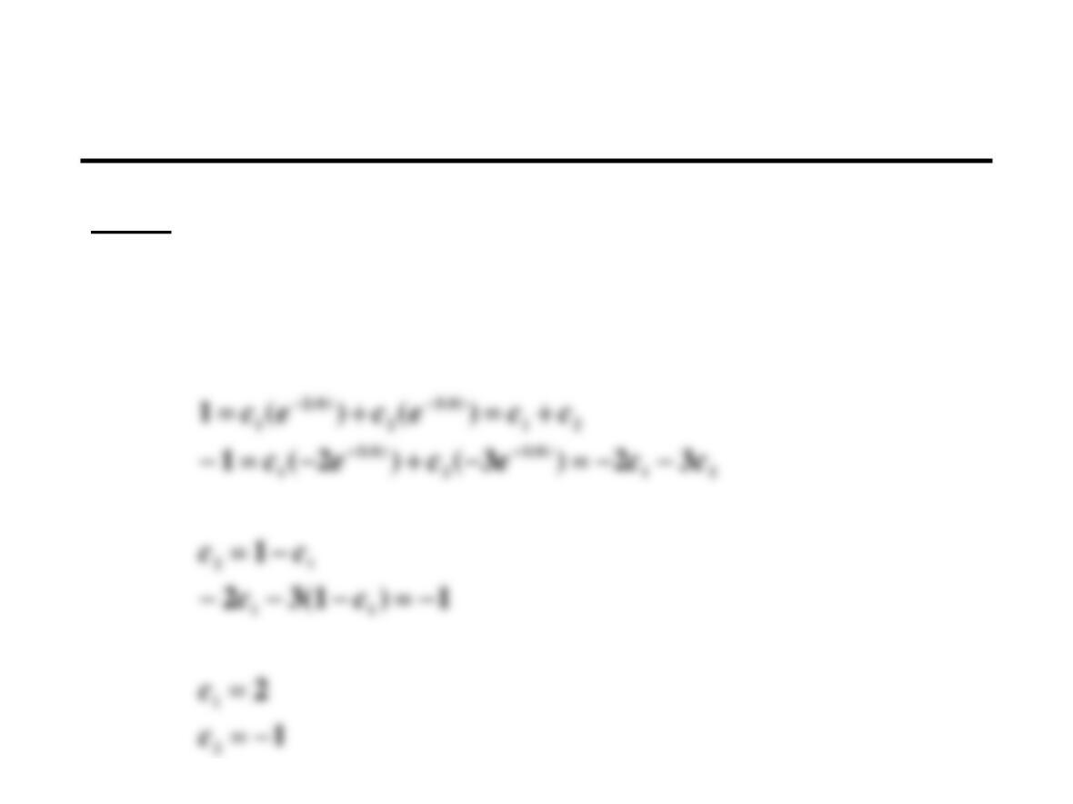
Step 4: Perform the integrations to determine the particular solution
)()(
))(()(),()(
)(3)(2
0
)(3)(2
0
t t tt
ttt
t
P
deedee
deeedgtKty
−−−−−−
−−−−−
=−
=−==
Kernel Method: Example (4)
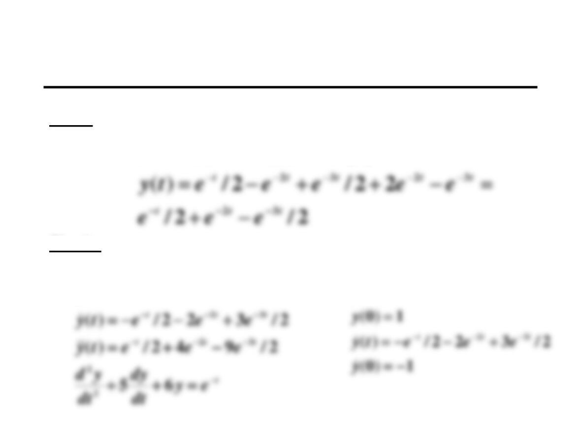
Step 5: Calculate the coefficients from
)0()0()0(
)0()0()0(
22110
22110
+==
+==
ycycyy
ycycyy
i
c
Kernel Method: Example (5)
Step 6: Calculate the final answer
Checks:
(1) Try the solution in the ODE: (2) Try the solution in initial conditions:
)()()()(
2211
P
tyctyctyty
++=
ttt
eeety
−−−
−+=
2/2/)(
32
2/2/)(
32
−+=
−−−
eeety
ttt

Second Order Linear Time-Invariant
Nonhomogeneous ODEs
Example for Undetermined Coefficients
(Trial & Error) Method
Undetermined Coefficients Method Example
Problem: Find the steady state solution to
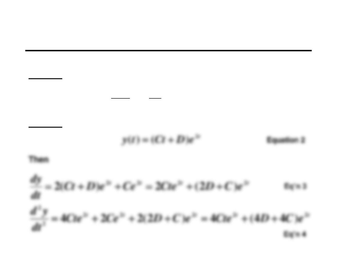
Solution: We try
t
tey
dt
dy
dt
yd 2
2
2
543 =++
Equation 1
Undetermined Coefficients Method Example (2)
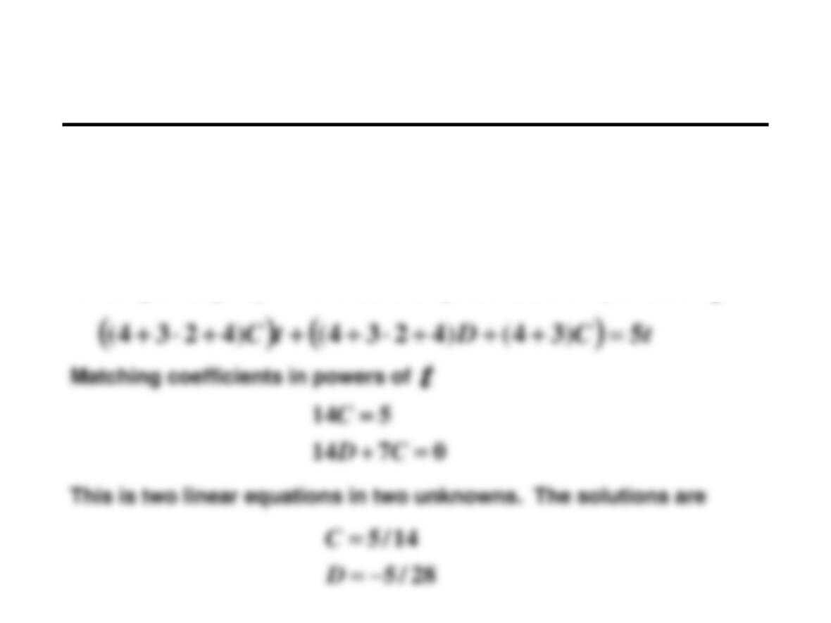
Substituting Equations 2, 3 and 4 into Equation 1:
Dividing through by and collecting coefficients in powers of
t
tttttt teeDCteCDCteeCDCte 222222 5)(4)2(23)44(4 =+++++++
t
e2
t
Undetermined Coefficients Method Example (3)
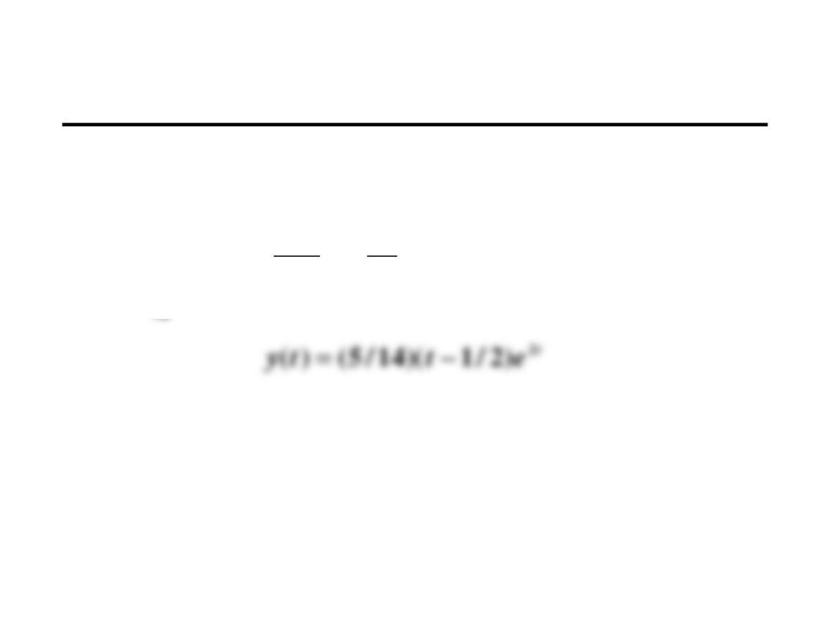
Hence the steady state solution to
is
t
tey
dt
dy
dt
yd 2
2
2
543 =++
Higher Order Linear ODEs
Quick survey – will address in more detail
later with state space representation
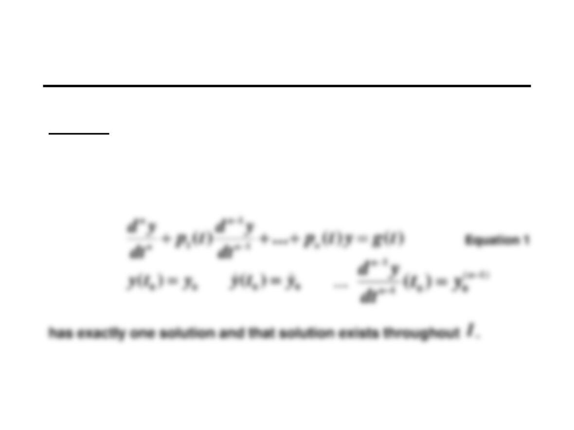
Existence and Uniqueness
Theorem:
Let the functions be continuous on the
open interval containing . Then the ODE
)(),(),...,(),(21 tgtptptp n
I
0
t
I