Applied Statistics and Probability for Engineers, 7th edition 2017
11-1
CHAPTER 11
Section 11-2
11.2.1 a)
01i i i
yx
= + +
2
6322.28
162674.2 2789.282
250
xx
S= − =
11.2.2 a)
Regression Analysis – Linear model: Y = a+bX
Dependent variable: SalePrice Independent variable: Taxes
——————————————————————————–
Standard T Prob.
Parameter Estimate Error Value Level
——————————————————————————–
Analysis of Variance
Source Sum of Squares Df Mean Square F-Ratio Prob. Level
Model 636.15569 1 636.15569 72.5563 .00000
Applied Statistics and Probability for Engineers, 7th edition 2017
b)
ˆ13.3202 3.32437(7.5) 38.253y= + =
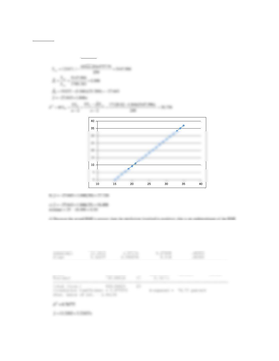
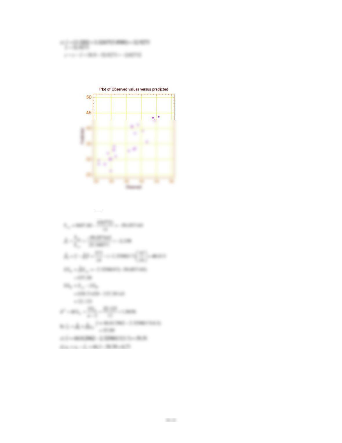
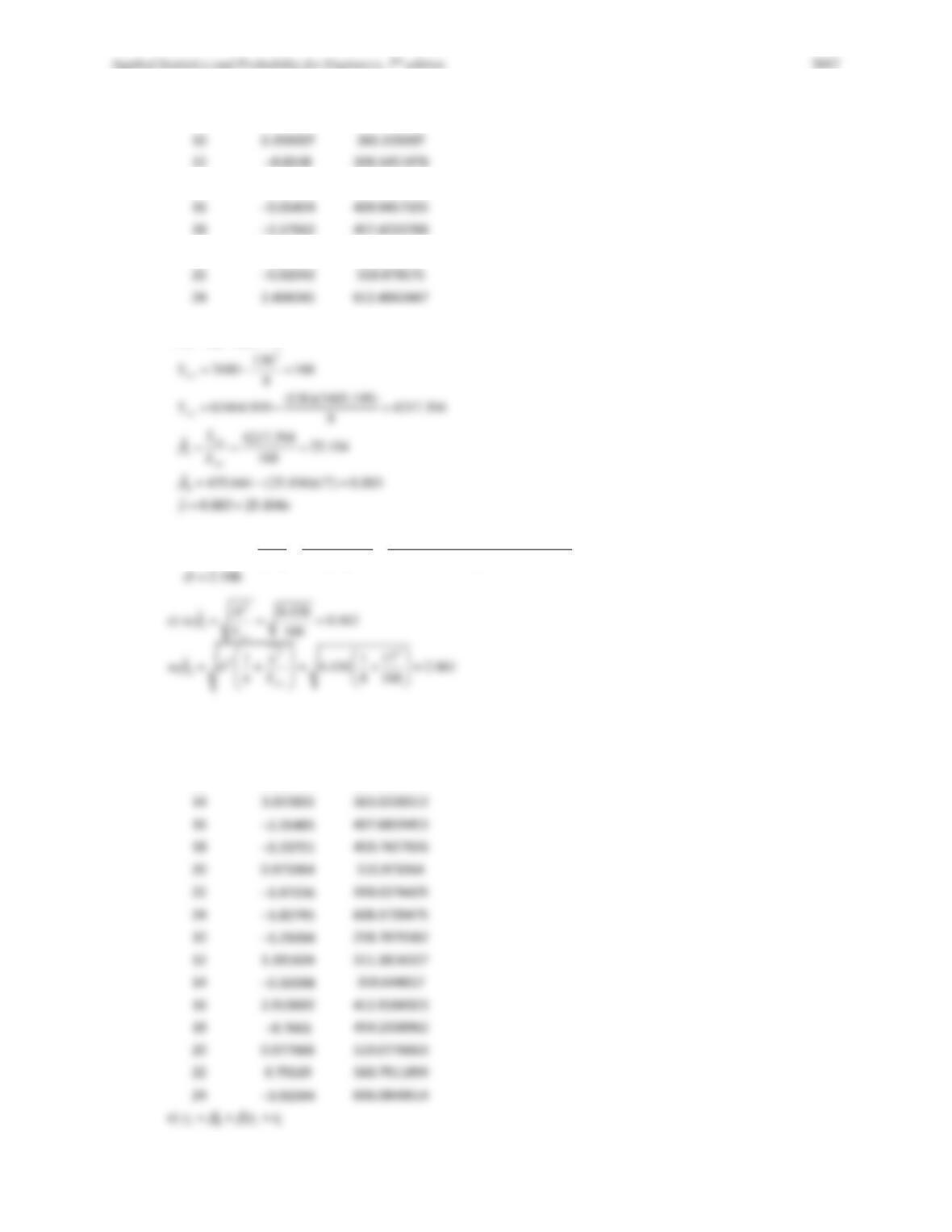
d) All the points would lie along a 45 degree line. That is, the regression model would estimate the values exactly. At
this point, the graph of observed vs. predicted indicates that the simple linear regression model provides a reasonable fit
to the data.
11.2.3 a)
01i i i
yx
= + +
2
43
157.42 25.348571
14
xx
S= − =
i i i
11-3
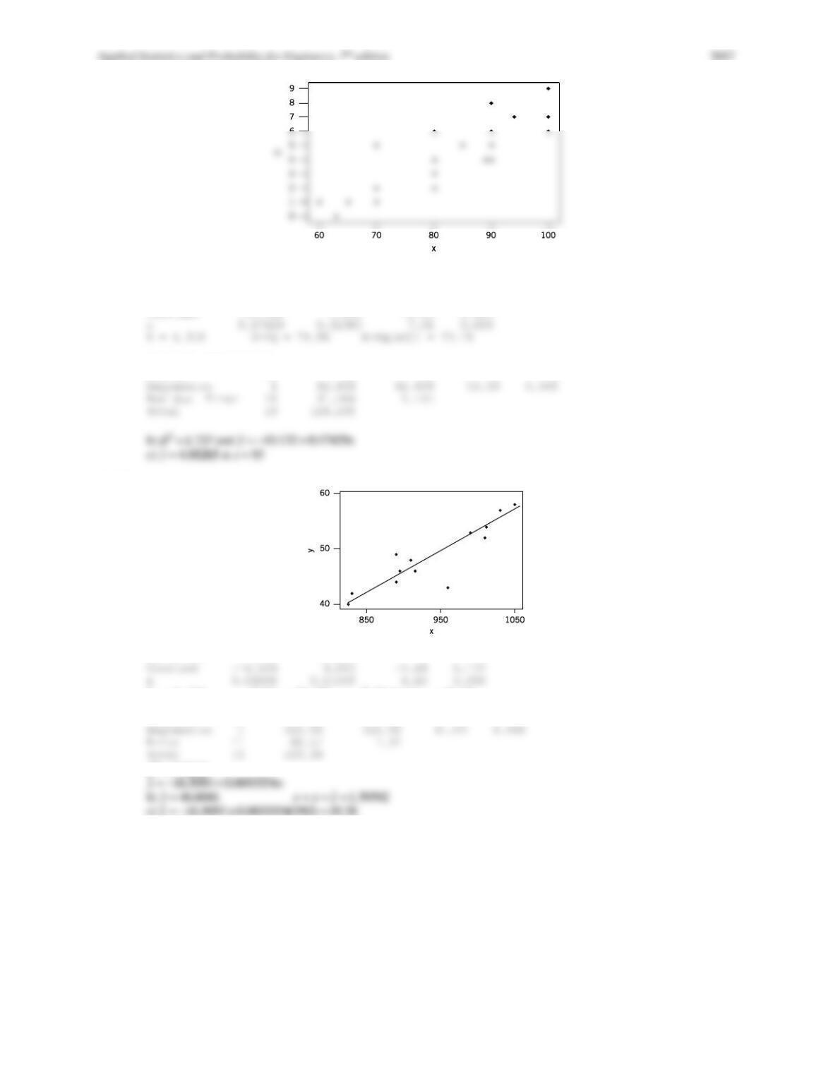
11.2.4 a)
Yes, a linear regression seems appropriate, but one or two points might be outliers.
Predictor Coef SE Coef T P
Constant -10.132 1.995 -5.08 0.000
Analysis of Variance
Source DF SS MS F P
11.2.5 a)
Predictor Coef StDev T P
S = 2.706 R-Sq = 80.0% R-Sq(adj) = 78.2%
Analysis of Variance
Source DF SS MS F P
2
ˆ7.3212
=
Applied Statistics and Probability for Engineers, 7th edition 2017
11-4
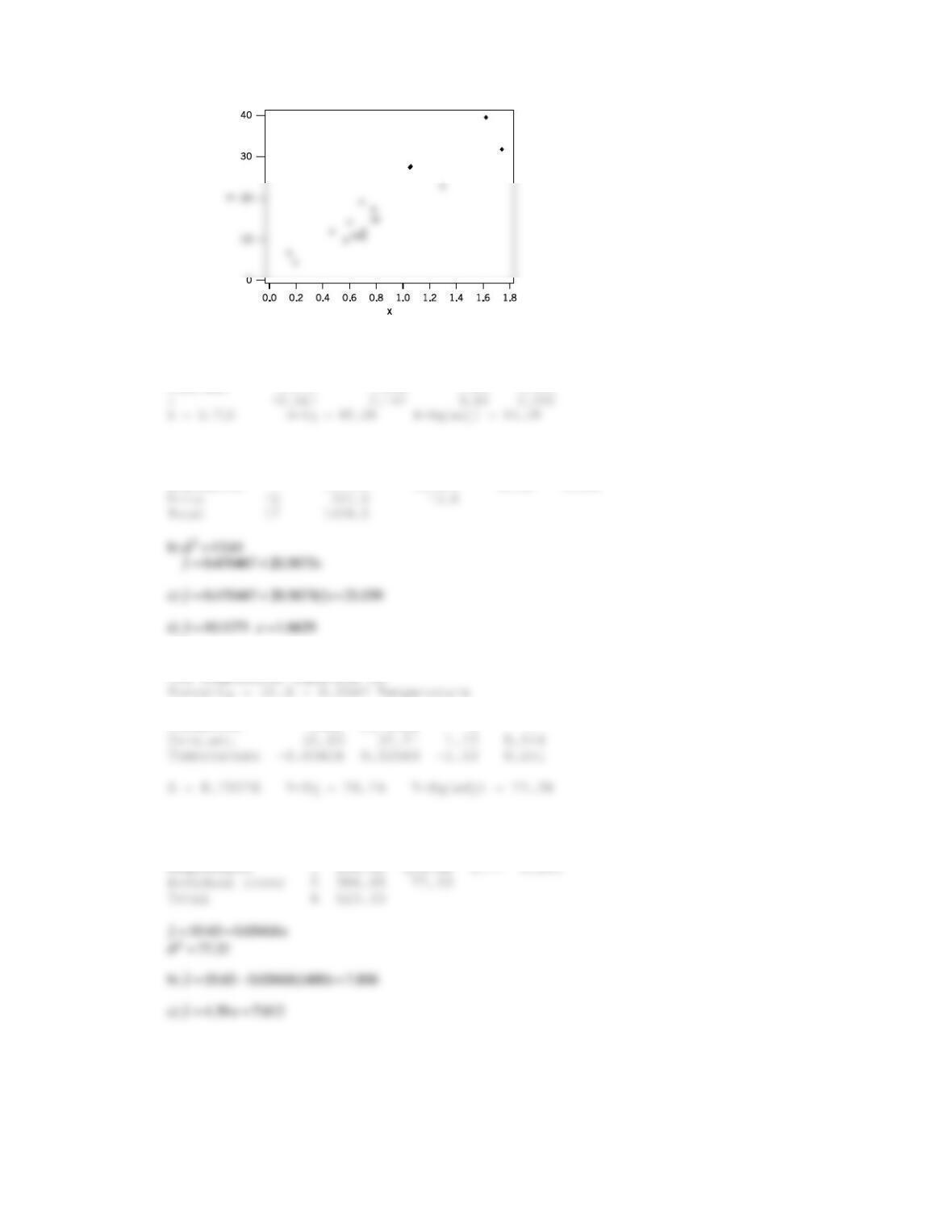
11.2.6 a)
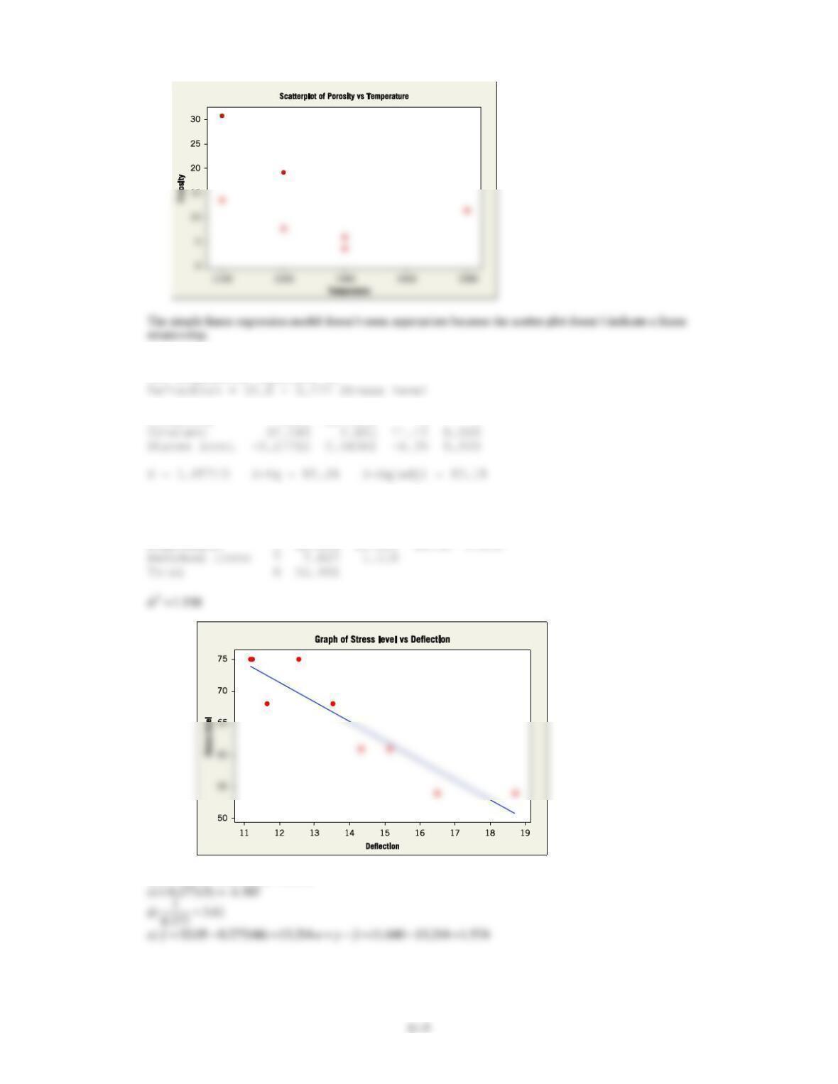
Yes, a simple linear regression model seems appropriate for these data.
Predictor Coef StDev T P
Constant 0.470 1.936 0.24 0.811
Analysis of Variance
Source DF SS MS F P
Regression 1 1273.5 1273.5 92.22 0.000
11.2.7 a)
The regression equation is
Predictor Coef SE Coef T P
Analysis of Variance
Source DF SS MS F P
Applied Statistics and Probability for Engineers, 7th edition 2017
d)
11.2.8 a)
The regression equation is
Predictor Coef SE Coef T P
Analysis of Variance
Source DF SS MS F P
Regression 1 45.154 45.154 40.38 0.000
b)
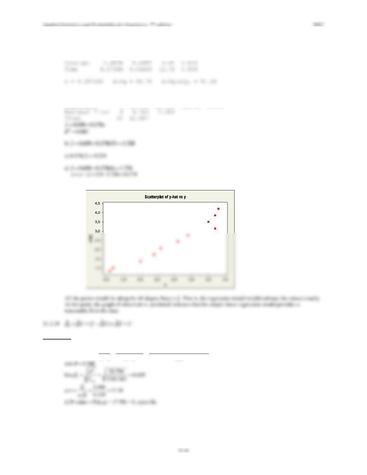
ˆ32.05 0.277(65) 14.045y= − =
11.2.9 a)
The regression equation is
BOD = 0.658 + 0.178 Time
Predictor Coef SE Coef T P
Analysis of Variance
Source DF SS MS F P
Regression 1 13.344 13.344 161.69 0.000
e)
Section 11-4
11.4.1 a)
1
2ˆ17128.82 1.846(5147.10)
ˆ30.756
2 2 248
T xy
E
E
SS S
SS
MS nn
−−
= = = = =
−−
11-7
11.4.2 Results will depend on the simulated errors. Example data are shown.
x
e
y
10
0.159207
260.159207
12
309.1451978
14
3.040714
363.0407136
18
457.4233788
20
3.050463
513.0504634
22
559.979575
24
2.404245
612.4042447
a)
01i i i
yx
= + +
b)
1
2ˆ105898.118 25.104(4217.394)
ˆ4.436
2 2 6
T xy
E
E
SS S
SS
MS nn
−−
= = = = =
−−
d) Results will depend on the simulated data. Example data are shown.
x
e
y
10
−3.81589
256.1841058
12
1.792464
311.792464
14
363.0228512
16
−2.31405
407.6859453
18
20
22
−1.97236
558.0276425
24
10
−1.29204
258.7079582
12
311.1816337
14
359.644017
16
412.9106923
18
459.2338962
20
0.077666
Applied Statistics and Probability for Engineers, 7th edition 2017
11-8
= − =
2
272
4960 336
16
xx
S
11.4.3 a)
00
0
0
ˆ12.857 12.4583
( ) 1.032
Tse
−
= = =
E
11.4.4 Refer to ANOVA for the referenced exercise.
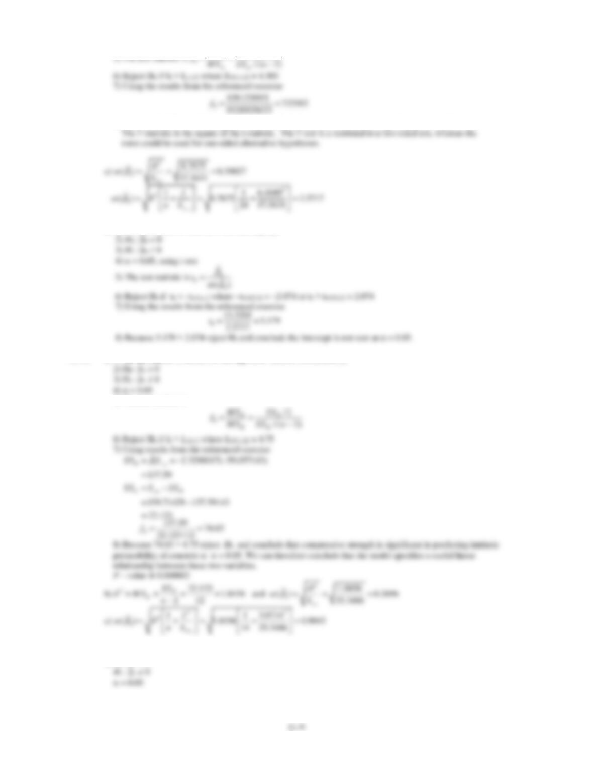
a) 1) The parameter of interest is the regressor variable coefficient, 1.
2) H0 : 1 = 0
Applied Statistics and Probability for Engineers, 7th edition 2017
/1
RR
M S SS
8) Because 72.5563 > 4.303, reject H0 and conclude the model is useful at a significance = 0.05.
d) 1) The parameter of interest is the intercept, 0.
11.4.5 a) 1) The parameter of interest is the regressor variable coefficient, 1
5) The test statistic is
11.4.6 Refer to the ANOVA for the referenced exercise
a) H0 : 1 = 0
11-10
53.50
f
=
b)
ˆ
( ) 0.0256613se
=
11.4.7 Refer to the ANOVA for the referenced exercise.
a) H0 : 1 = 0
b)
β1
ˆ
( ) 0.0104524se =
11.4.8 Refer to the ANOVA for the referenced exercise
a) H0 : 1 = 0
b) P-value < 0.00001
Applied Statistics and Probability for Engineers, 7th edition 2017
11-11
d)
00
:0H=
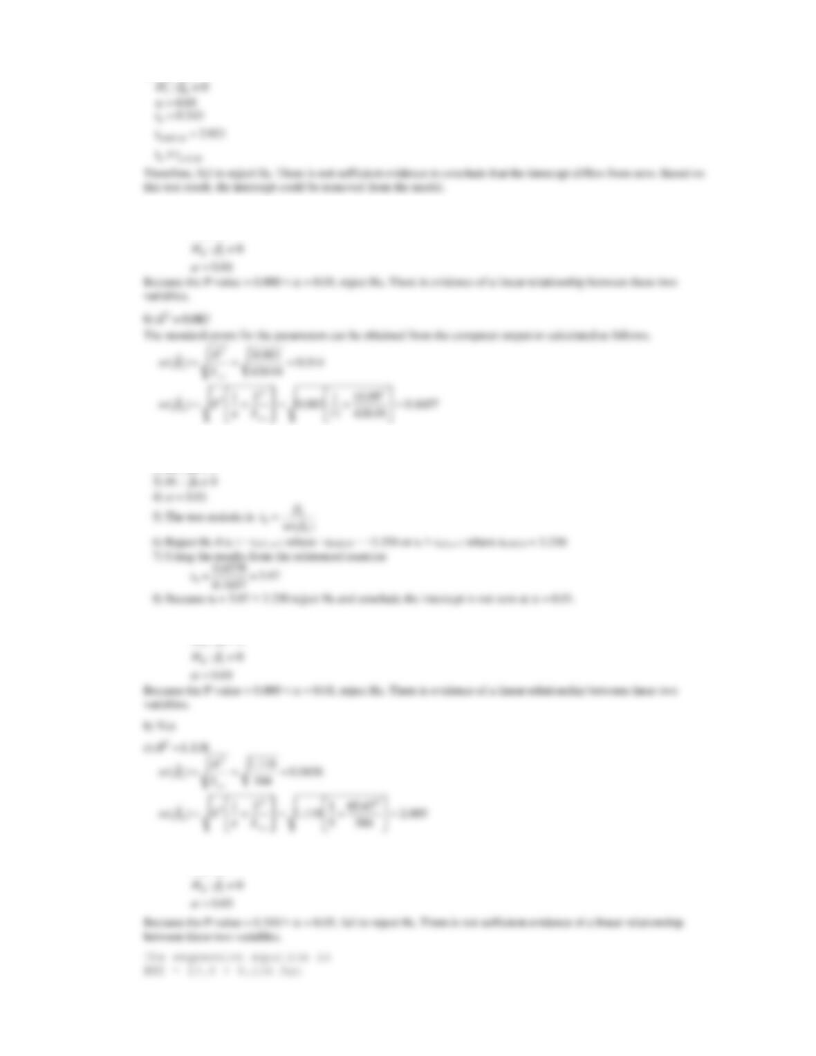
11.4.9 a) Refer to the ANOVA from the referenced exercise.
01
:0
H
=
c)
1) The parameter of interest is the intercept 0.
2) H0 :
0 = 0
11.4.10 a) Refer to the ANOVA for the referenced exercise.
01
:0
H
=
11.4.11 a)
01
:0
H
=
Applied Statistics and Probability for Engineers, 7th edition 2017
11-12
Predictor Coef SE Coef T P
Constant 13.820 9.141 1.51 0.174
Sections 11-5 and 11-6
11.6.1
1
5147.996
ˆ1.846
2789.282
xy
xx
S
S
= = =
a) 95% confidence interval on
1
1 / 2, 2 1
ˆˆ
()
n
t se
−
b) 95% confidence interval for the mean when BMI is 25
ˆ27.643 1.846(25) 18.498
= − + =
c) 95% prediction interval on x0 = 25.0
( )
2
0
2
0.025,248
1
ˆˆ
1
xx
xx
yt nS
−
+ +
11.6.2 Regression Analysis: Price versus Taxes
Applied Statistics and Probability for Engineers, 7th edition 2017
11-13
Constant 13.320 2.572 5.18 0.000
Taxes 3.3244 0.3903 8.52 0.000
Analysis of Variance
Source DF SS MS F P
Regression 1 636.16 636.16 72.56 0.000
d)
2
1 (7.5 6.40492)
38.253 (2.074) 8.76775 1 24 57.563139
−
+ +
11.6.3 t/2,n-2 = t0.025,12 = 2.179
b) 95% confidence interval on
c) 95% confidence interval on when x0 = 2.5
d) 95% on prediction interval when x0 = 2.5
11.6.4 a) 0.11756 ≤
1 ≤ 0.22541
Applied Statistics and Probability for Engineers, 7th edition 2017
b) −14.3002 ≤
0 ≤ −5.32598
11.6.5 a) 0.03689 ≤
1 ≤ 0.10183
11.6.6 a) 14.3107 ≤
1 ≤ 26.8239
d)
2
1 (1 0.806111)
21.038 (2.921) 13.8092 1 18 3.01062
−
+ +
11.6.7 Refer to the computer output in the referenced exercise.
/2, 2 0.005,9 3.250
n
tt
−==
a) 99% confidence interval for
ˆ
11-15
11.6.8 t/2,n−2 = t0.025,5 = 2.571
a) 95% confidence interval on
1
ˆ
b) 95% confidence interval on
0
0 /2, 2 0
ˆˆ
()
n
t se
−
c) 95% confidence interval for the mean length when x=1500:
ˆ55.63 0.034(1500) 4.63
= − =
Section 11-7
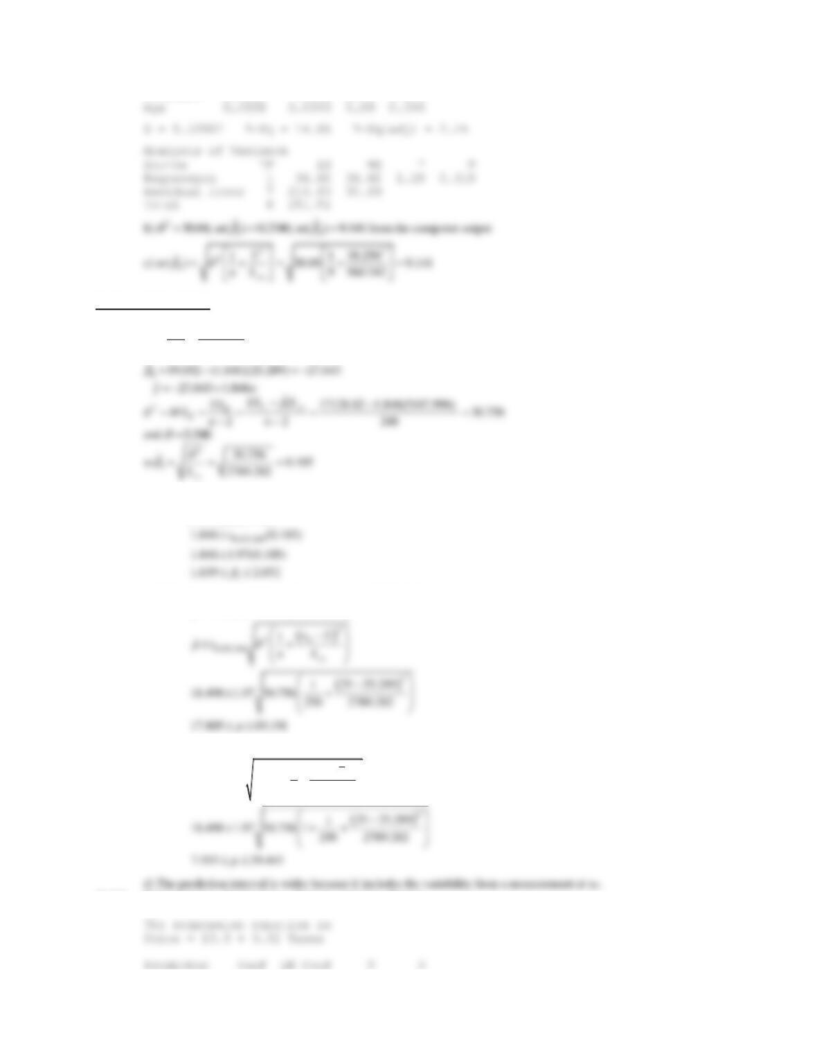
11.7.1
Results will depend on the simulated errors. Example data follow.
x
e
y
553.777
Applied Statistics and Probability for Engineers, 7th edition 2017
11-16
a)
01
i i i
yx
= + +
b)
1
2ˆ154778.884 30.343(5097.583)
ˆ17.364
2 2 6
T xy
E
E
SS S
SS
MS nn
−−
= = = = =
−−
d) Results will depend on the simulated errors. Example data follow.
x
e
y
10
−1.01617
308.98383
14
−9.26768
420.73232
18
−5.13715
544.86285
22
−1.71362
668.28638
26
793.777
30
−4.28057
905.71943
34
−4.05776
1025.9422
38
1152.3371
e)
1
ˆ30.171(20275.165) 611729.664
R xy
SS S
= = =
11-17
11.7.2
Results depend on the simulated errors. Example data follow for the model y = 10 + 30x.
Model y = 10 + 30x
x
e
y
308.4957
14
1.836897
431.8369
16
0.35073
490.3507
18
0.80104
550.801
609.7384
669.2921
24
0.36672
730.3667
a)
01i i i
yx
= + +
b)
1
2ˆ151672.357-30.046(5047.743)
ˆ1.233
2 2 6
T xy
E
E
SS S
SS
MS nn
−
= = = = =
−−
c)
1
ˆ30.046(5047.743) 151664.958
R xy
SS S
= = =
d) Results will depend on the simulated errors. Example data follow.
x
e
y
10
−1.50427
308.4957
14
−0.80622
429.1938
18
551.8369
22
670.3507
26
30
−0.26163
909.7384
34
−0.70788
1029.292
38
1150.367
01i i i
Applied Statistics and Probability for Engineers, 7th edition 2017
11-18
2
192
5280 672
8
xx
S
= − =
e)
1
ˆ30.023(20175.487) 605729.56
R xy
SS S
= = =
11.7.4 Use the results from the referenced exercise to answer the following questions.
a) SalePrice Taxes Predicted Residuals
25.9 4.9176 29.6681073 -3.76810726
29.5 5.0208 30.0111824 -0.51118237
Applied Statistics and Probability for Engineers, 7th edition 2017
11-19
Applied Statistics and Probability for Engineers, 7th edition 2017
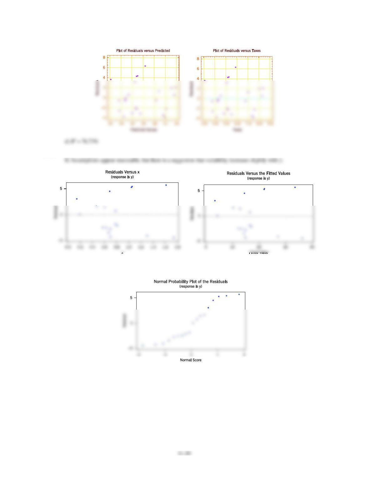
c) There are no serious departures from the assumption of constant variance. This is evident by the random pattern of
the residuals.
11.7.5 a) R2 = 85.22%
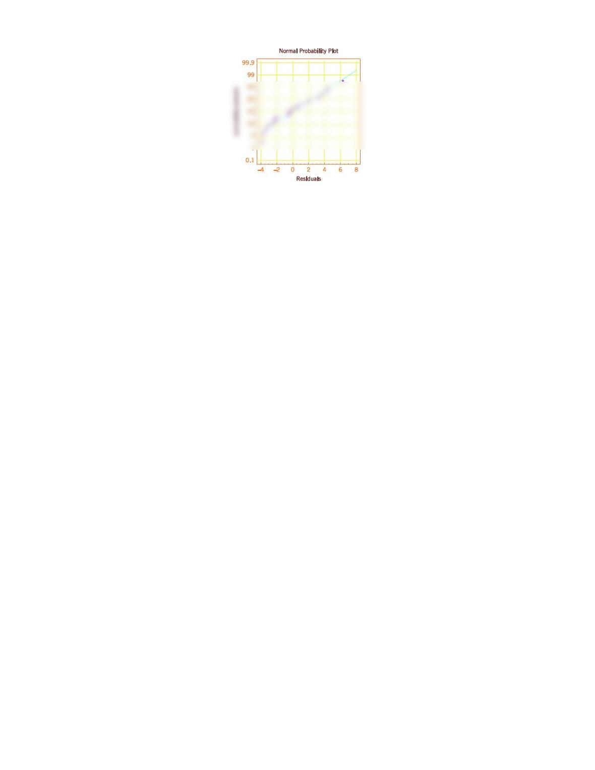
c) Normality assumption may be questionable. There is some “bending” away from a line in the tails of the normal
probability plot.