Applied Statistics and Probability for Engineers, 7th edition 2017
11-32
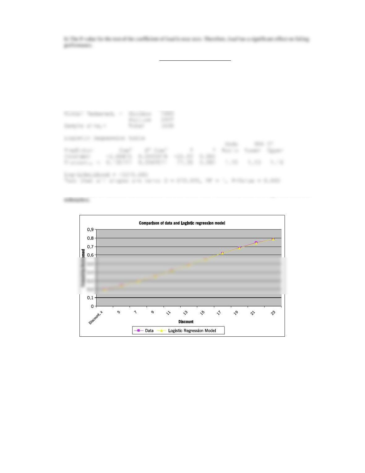
11.10.3 a) The fitted logistic regression model is
1
ˆ
1 exp[ ( 2.08475 0.13573 )]
yx
=+ − − +
The computer results are shown below.
Binary Logistic Regression: Number Redee, Sample size, versus Discount, x
Link Function: Logit
Response Information
Variable Value Count
b) The P-value for the test of the coefficient of discount is near zero. Therefore, discount has a significant effect on
c)
Applied Statistics and Probability for Engineers, 7th edition 2017
11-33
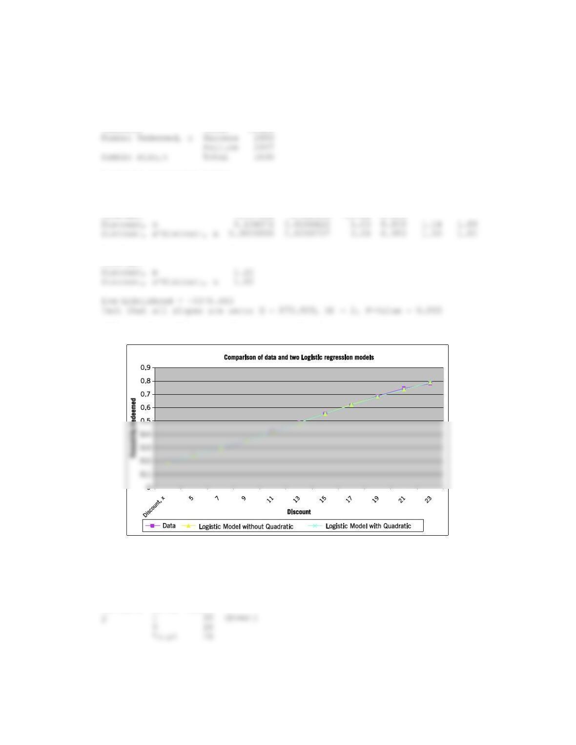
d) The P-value of the quadratic term is 0.95 > 0.05, so we fail to reject the null hypothesis of the quadratic coefficient at
the 0.05 level of significance. There is no evidence that the quadratic term is required in the model. The computer
results are shown below.
Binary Logistic Regression: Number Redee, Sample size, versus Discount, x
Link Function: Logit
Response Information
Variable Value Count
Logistic Regression Table
95%
Odds CI
Predictor Coef SE Coef Z P Ratio Lower
Constant -2.07422 0.185045 -11.21 0.000
Predictor Upper
Constant
e) The expanded model does not visually provide a better fit to the data than the original model.
11.10.4 a) The computer results are shown below.
Binary Logistic Regression: y versus Income x1, Age x2
Link Function: Logit
Response Information
Variable Value Count
Applied Statistics and Probability for Engineers, 7th edition 2017
11-34
Logistic Regression Table
Odds 95% CI
Predictor Coef SE Coef Z P Ratio Lower Upper
Constant -7.04706 4.67416 -1.51 0.132
b) Because the P-value = 0.036 < = 0.05 we can conclude that at least one of the coefficients (of income and age) is
not equal to zero at the 0.05 level of significance. The individual z-tests do not generate P-values less than 0.05, but this
c) The odds ratio is changed by the factor exp(1) = exp(0.0000738) = 1.00007 for every unit increase in income with
age held constant. Similarly, odds ratio is changed by the factor exp(1) = exp(0.987886) = 2.686 for every unit
d) At x1 = 45000 and x2 = 5 from part (a)
Binary Logistic Regression: y versus Income x1, Age x2
Link Function: Logit
Response Information
Variable Value Count
Logistic Regression Table
Odds 95% CI
Predictor Coef SE Coef Z P Ratio Lower Upper
Constant 0.314351 6.39401 0.05 0.961
11.10.5
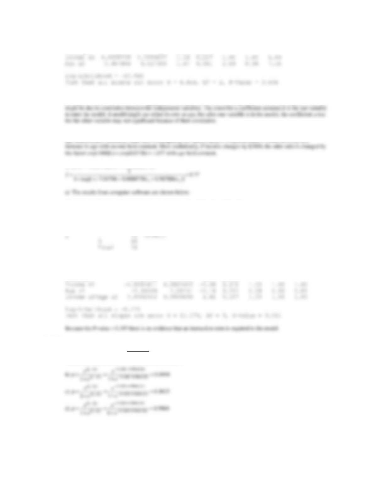
a) The logistic function is
01
01
1
x
x
e
e
+
+
=+
. From a plot or from the derivative, this is a monotonic increasing function of x.
Therefore, the probability increases as a function of x.
Applied Statistics and Probability for Engineers, 7th edition 2017
e)
Supplemental Exercises
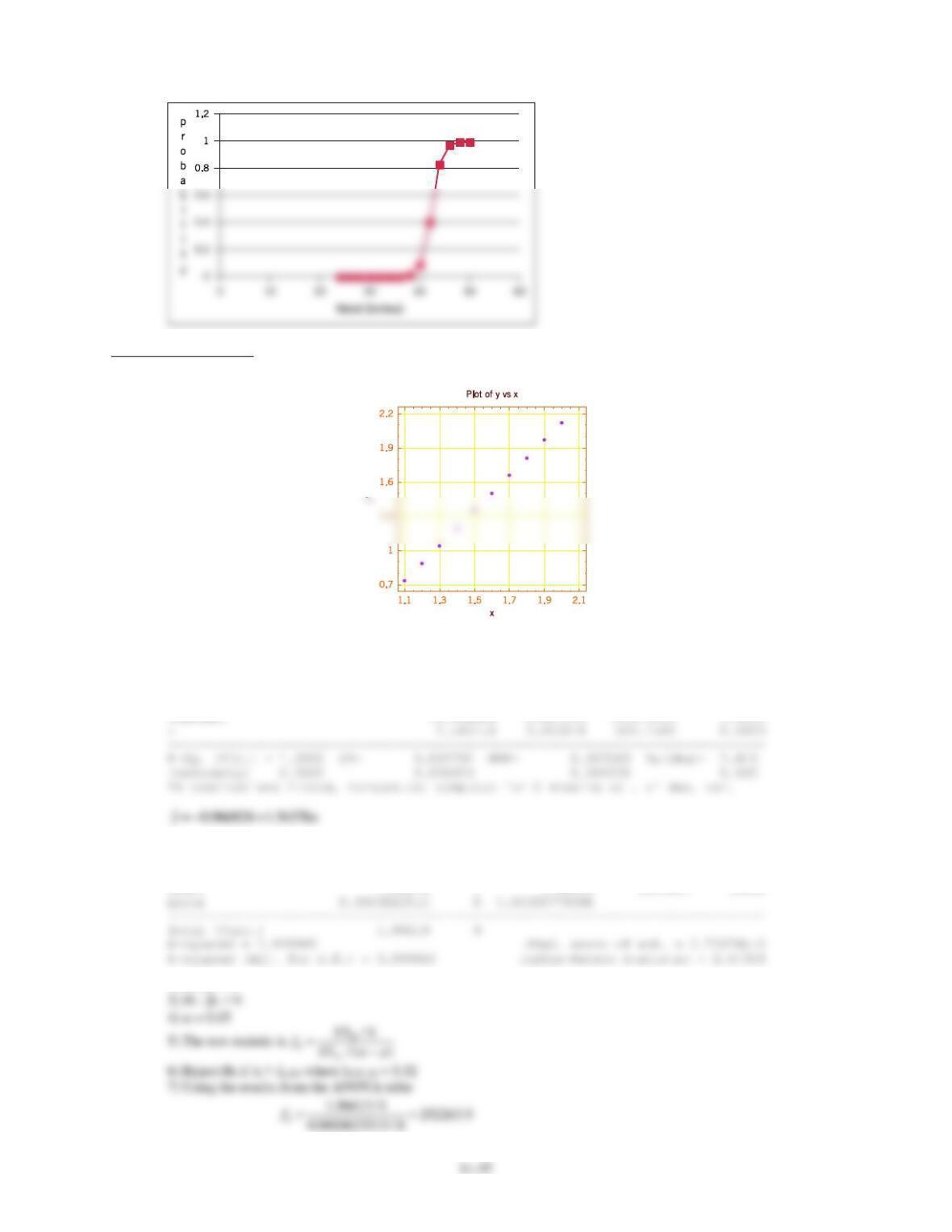
11.S7 a)
Yes, a linear relationship seems plausible.
b)
Model fitting results for: y
Independent variable coefficient std. error t-value sig.level
CONSTANT -0.966824 0.004845 -199.5413 0.0000
c)
Analysis of Variance for the Full Regression
Source Sum of Squares DF Mean Square F-Ratio P-value
Model 1.96613 1 1.96613 252264. .0000
2)H0 : 1 = 0
11-36
8) Because 252264 > 5.32 reject H0 and conclude that the regression model is significant at = 0.05.
P-value ≈ 0
d)
95 percent confidence intervals for coefficient estimates
——————————————————————————–
Estimate Standard error Lower Limit Upper Limit
e) 2) H0 : 0 = 0
5) The test statistic is
0
0
ˆ
ˆ
()
tse
=
11.S8 a)
1 1 1
ˆˆ
()
n n n
i i i i
i i i
y y y y
= = =
− = −
and
01
ˆˆ
ii
y n x
=+
from the normal equations
Then,
b)
1 1 1
ˆˆ
()
n n n
i i i i i i i
i i i
y y x y x y x
= = =
− = −
c)
1
1ˆ
n
i
i
yy
n=
=
01
ˆˆ
ˆ()yx
=+
11.S9
ˆ1.2232 0.5075yx
=+
where y* = 1/y. No, the model does not seem reasonable.
Applied Statistics and Probability for Engineers, 7th edition 2017
11-37
0
12.872
f
=
f)
11.S11
ˆ4.5755 2.2047yx=+
, r = 0.992, R2 = 98.40%
11.S12 a)
Applied Statistics and Probability for Engineers, 7th edition 2017
11-38
b) The regression equation is
ˆ193 15.296yx=− +
Analysis of Variance
Source DF SS MS F P
Fail to reject Ho. We do not have evidence of a relationship. Therefore, there is not sufficient evidence to conclude that
c) 95% CI on 1
1 /2, 2 1
ˆˆ
()
n
t se
−
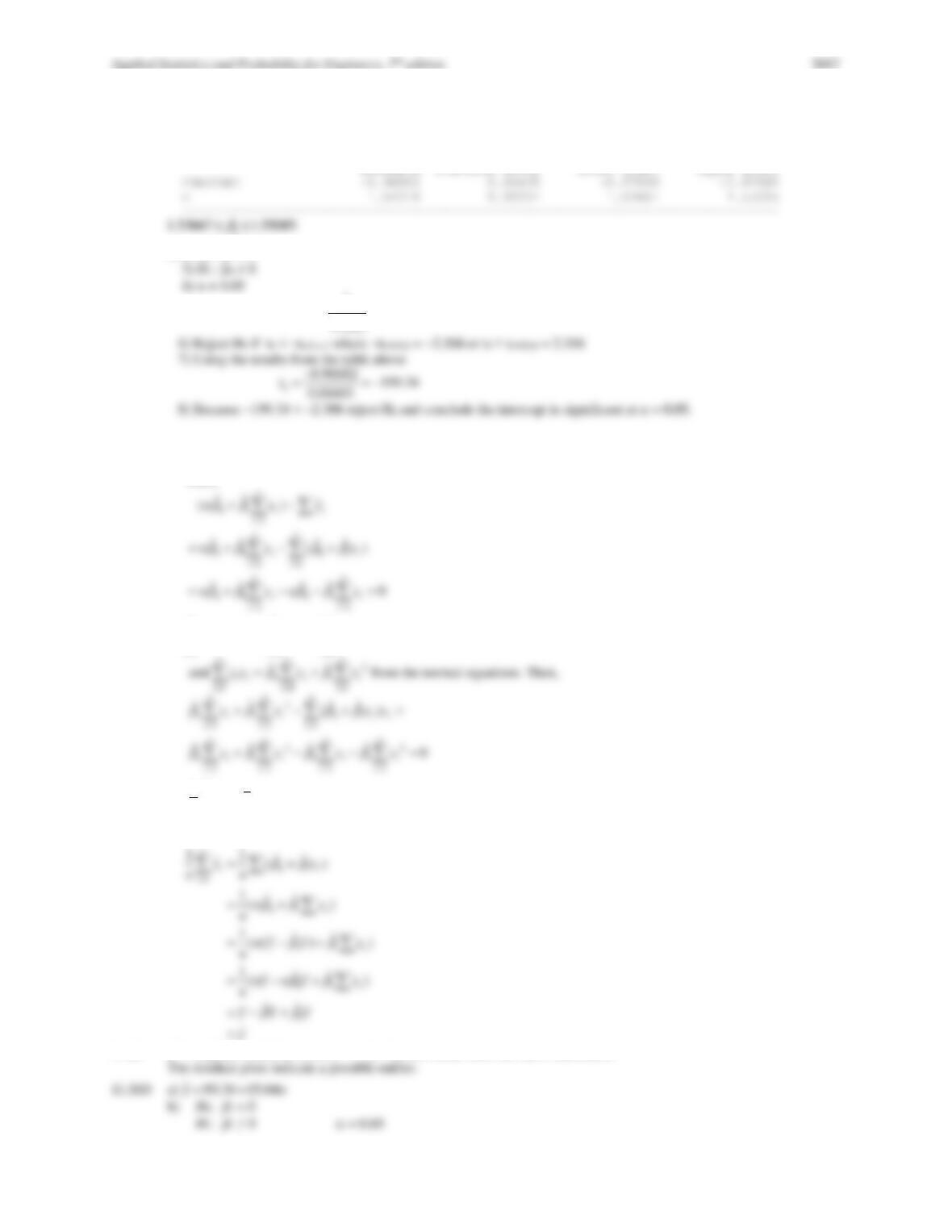
d) The normality plot of the residuals is satisfactory. However, the plot of residuals versus run order exhibits a strong
downward trend. This could indicate that there is another variable should be included in the model and it is one that
changes with time.
11.S13 a)
c)
Analysis of Variance
Source DF SS MS F P
Regression 1 0.03691 0.03691 1.64 0.248
Applied Statistics and Probability for Engineers, 7th edition 2017
11-39
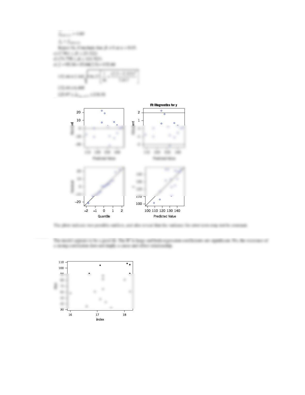
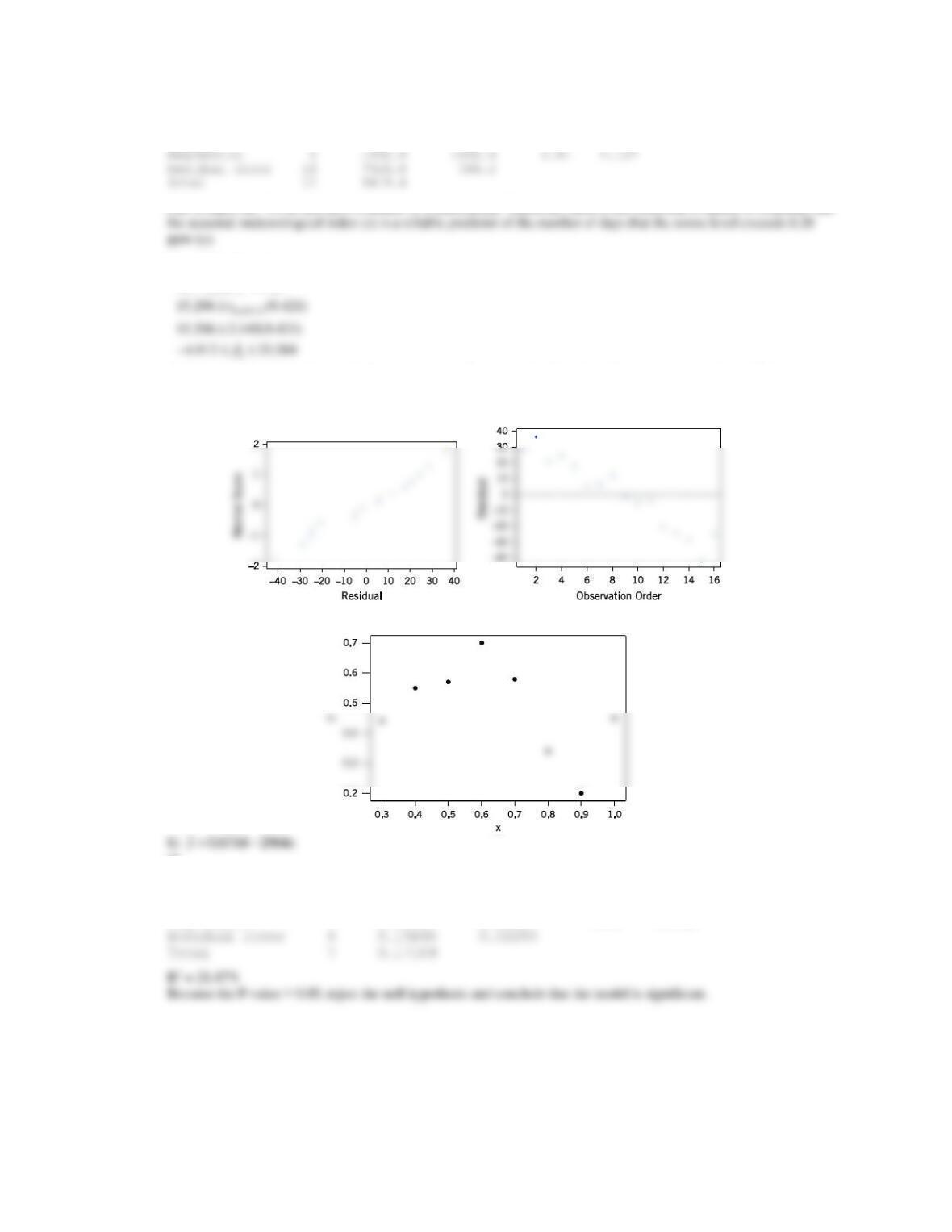
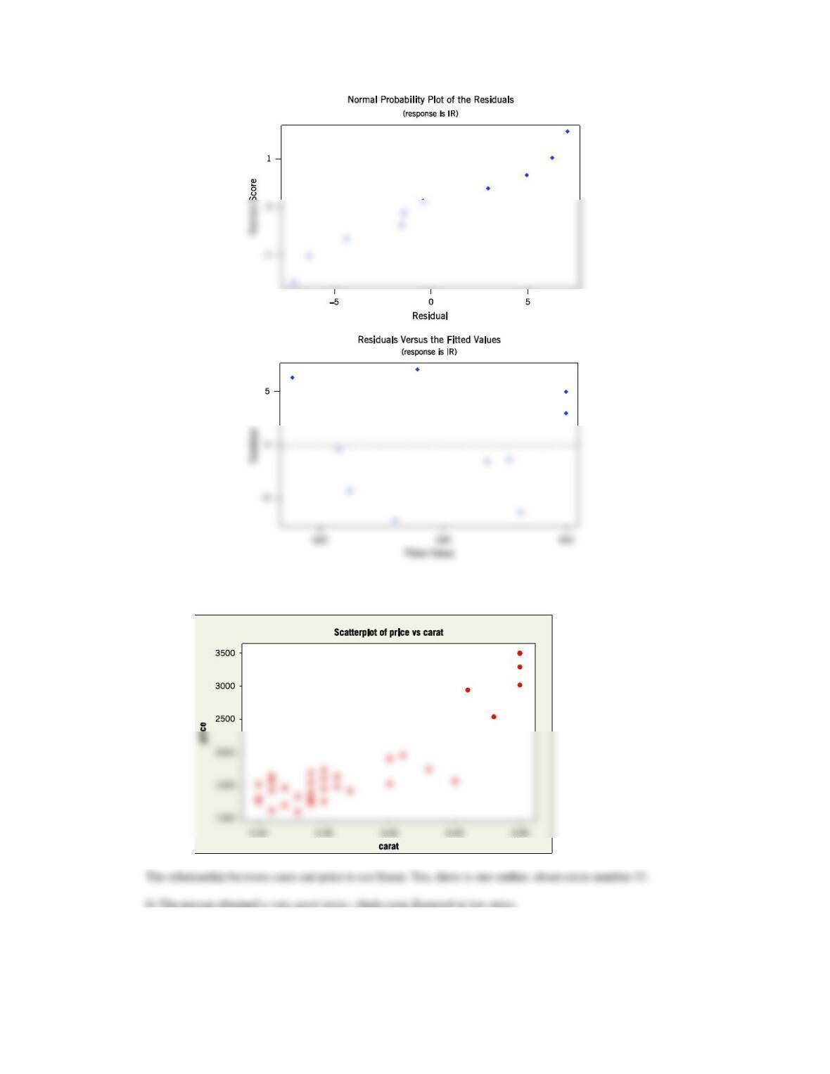
d) There appears to be curvature in the data. There is a dip in the middle of the normal probability plot and the plot of
the residuals versus the fitted values shows curvature.
11.S14 a)
b)
ˆ33.3 0.9636yx=+
c) Predictor Coef SE Coef T P
Analysis of Variance
Source DF SS MS F P
Regression 1 584.62 584.62 19.79 0.002
Reject the null hypothesis and conclude that the model is significant. Here 77.3% of the variability is explained by the
model.
d) H0 : 1 = 1
Applied Statistics and Probability for Engineers, 7th edition 2017
11-40
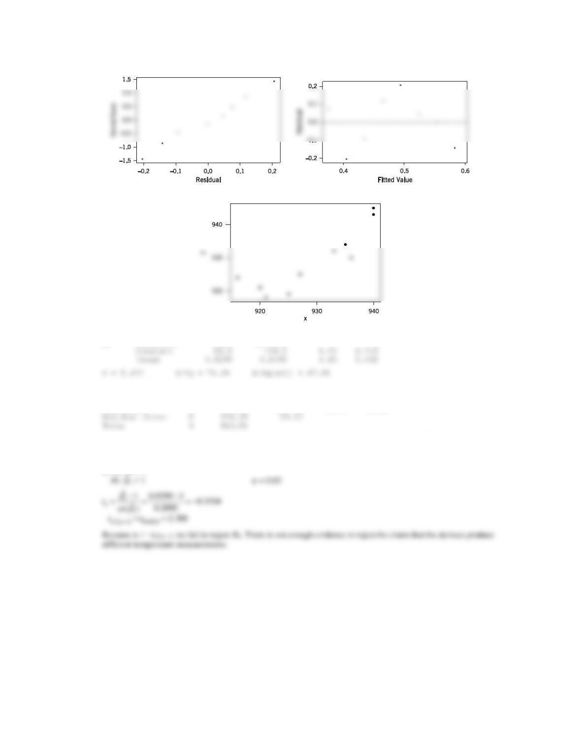
e) The residual plots to not reveal any major problems.
11.S15 a)
Applied Statistics and Probability for Engineers, 7th edition 2017
11-41
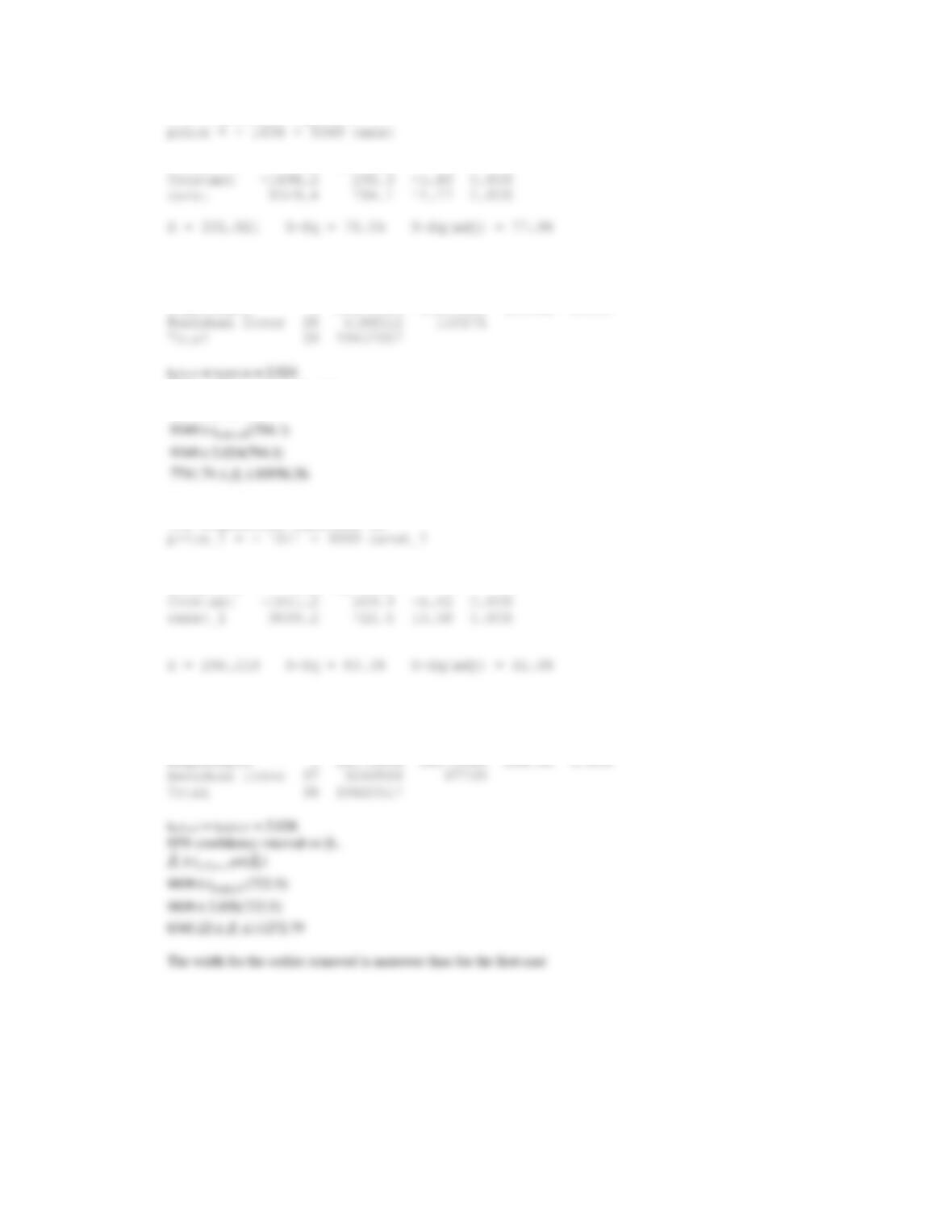
c) All the data
The regression equation is
Predictor Coef SE Coef T P
Analysis of Variance
Source DF SS MS F P
Regression 1 15270545 15270545 138.61 0.000
95% confidence interval on 1
1 / 2, 2 1
ˆˆ
()
n
t se
−
With unusual data omitted
The regression equation is
Predictor Coef SE Coef T P
Analysis of Variance
Source DF SS MS F P