Applied Statistics and Probability for Engineers, 7th edition 2017
11-21
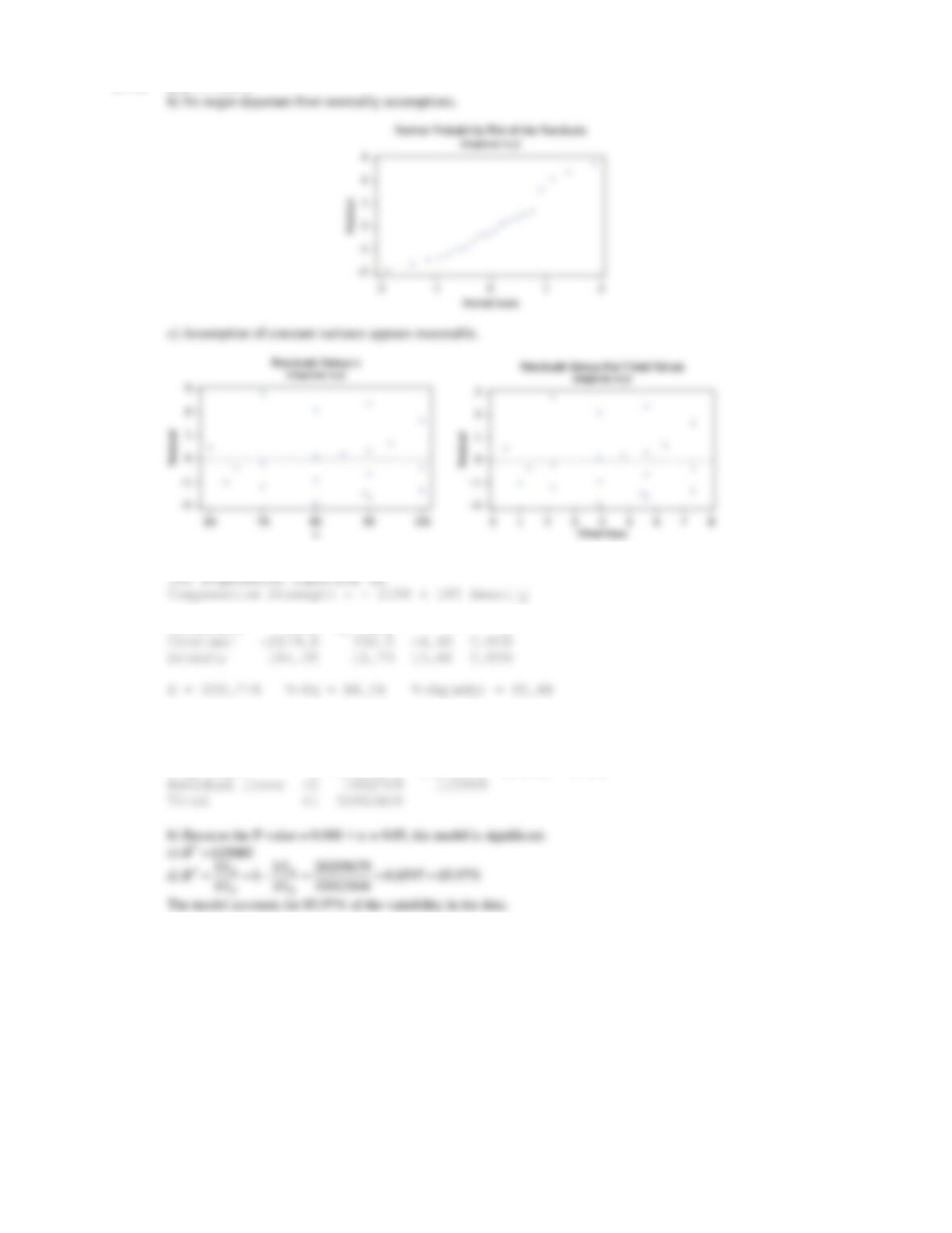
11.7.6 a) R2 = 71.27%
11.7.7 a)
Predictor Coef SE Coef T P
Analysis of Variance
Source DF SS MS F P
Regression 1 28209679 28209679 245.15 0.000
Applied Statistics and Probability for Engineers, 7th edition 2017
11-22
e)
f)
11.7.8 a)
b) H0 :
1 = 0 H1 :
1 ≠ 0 = 0.05
Applied Statistics and Probability for Engineers, 7th edition 2017
11-23
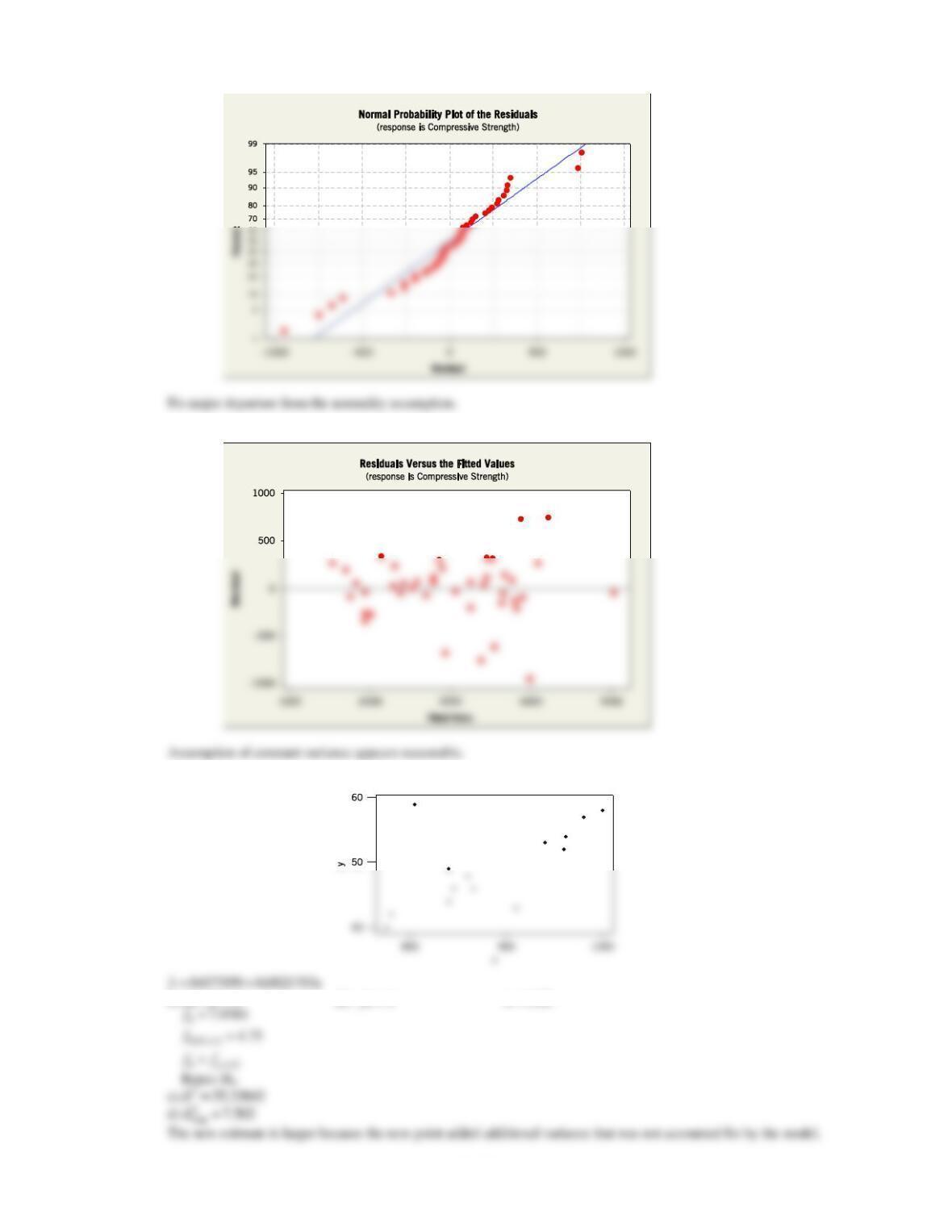
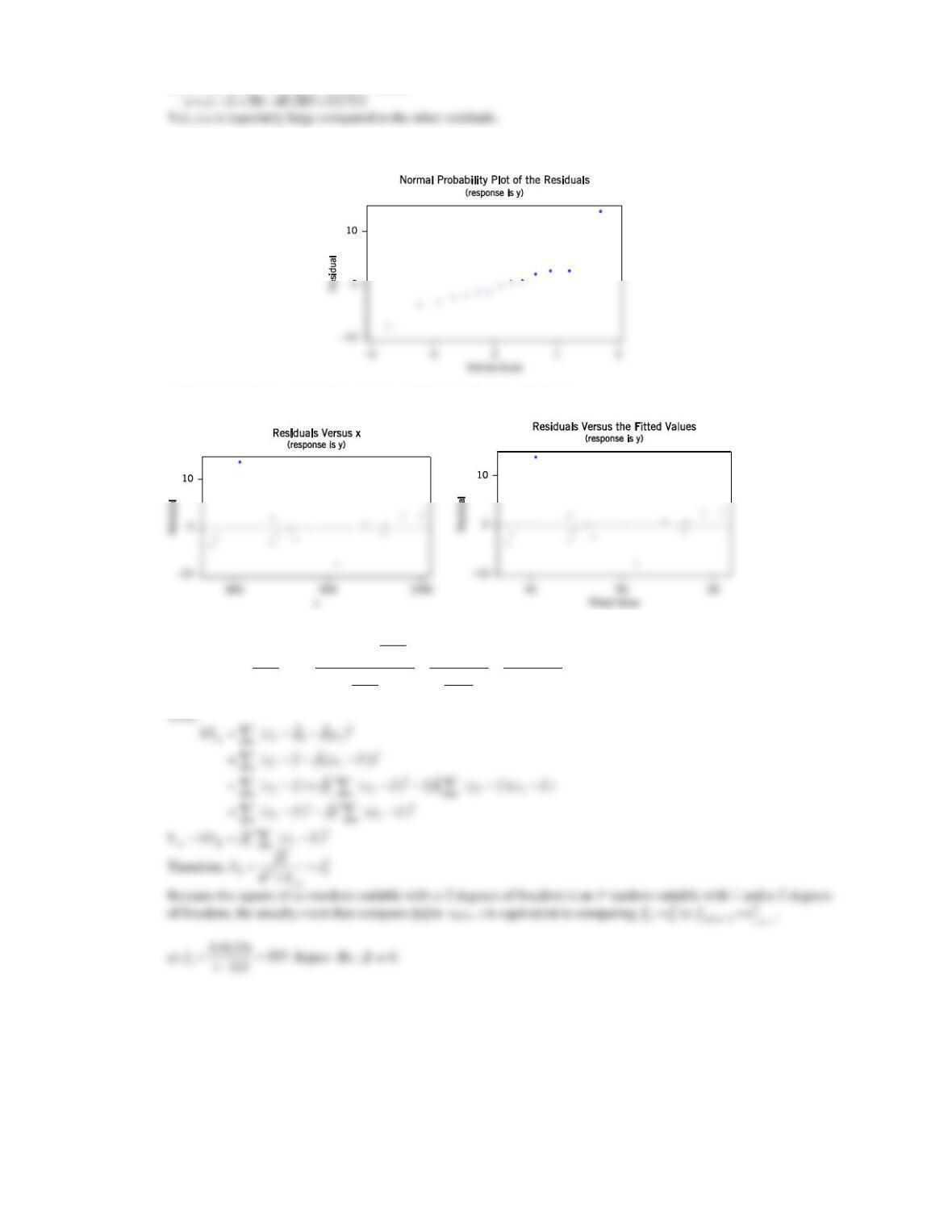
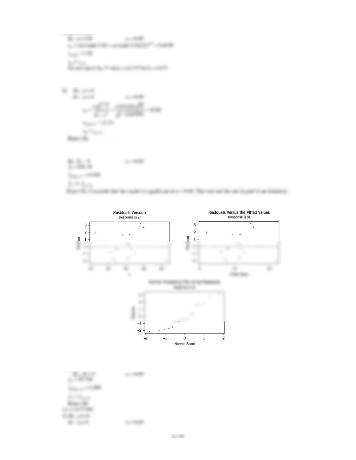
e)
ˆ0.677559 0.0521753(855) 45.287y= + =
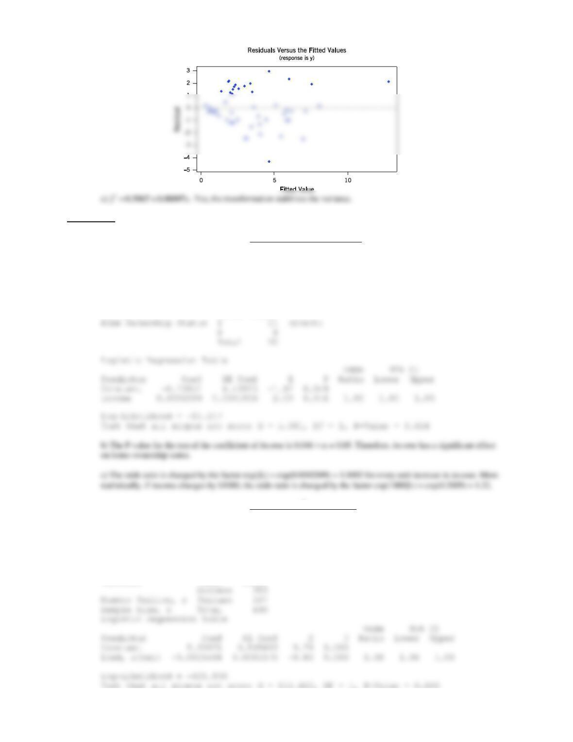
f) The one added point is an outlier and the normality assumption is not as valid with the point included.
g) Constant variance assumption appears valid except for the added point.
11.7.9 Using
=−
21,
E
yy
SS
RS
02
( 2) 1
ˆ
2
E
yy yy E yy E
EE
yy
SS
nSS SS S SS
FSS S S
Sn
−−
−−
= = =
−
Applied Statistics and Probability for Engineers, 7th edition 2017
11-24
b) Because f0.05,1,23 = 4.28, H0 is rejected if
2
2
23 4.28
1
R
R
−
11.7.10 For two random variables X1 and X2,
1 2 1 2 1 2
( ) ( ) ( ) 2Cov( , )V X X V X V X X X+ = + +
Then,
ˆ ˆ ˆ
( ) ( ) ( ) 2Cov( , )
i i i i i i
V Y Y V Y V Y Y Y
− = + −
a) Because ei is divided by an estimate of its standard error (when
2 is estimated by
2
ˆ
), ri has approximately unit
Section 11-8
11.8.1 a) H0 :
= 0
b) H0 :
= 0.5
c)
.025 .025
tanh arctanh 0.8 tanh arctanh 0.8+
17 17
zz
−
11.8.2 n = 25 r = 0.83

Applied Statistics and Probability for Engineers, 7th edition 2017
11-25
Applied Statistics and Probability for Engineers, 7th edition 2017
11.8.3 a) r = 0.933203
c)
ˆ0.72538 0.498081yx=+
H0 : 1 = 0
d) No problems with model assumptions are noted.
11.8.4 a)
ˆ69.1044 0.419415yx=+
b) H0 :
1 = 0
11-27
0
0.77349 24 5.9787
1 0.5983
t
==
−
e) H0 :
= 0.6
11.8.5 a)
Predictor Coef SE Coef T P
Analysis of Variance
Source DF SS MS F P
Regression 1 1493.7 1493.7 70.88 0.000
Applied Statistics and Probability for Engineers, 7th edition 2017
11-28
d)
/2 /2
tanh arctan h tanh arctan h
33
zz
rr
nn
− +
−−
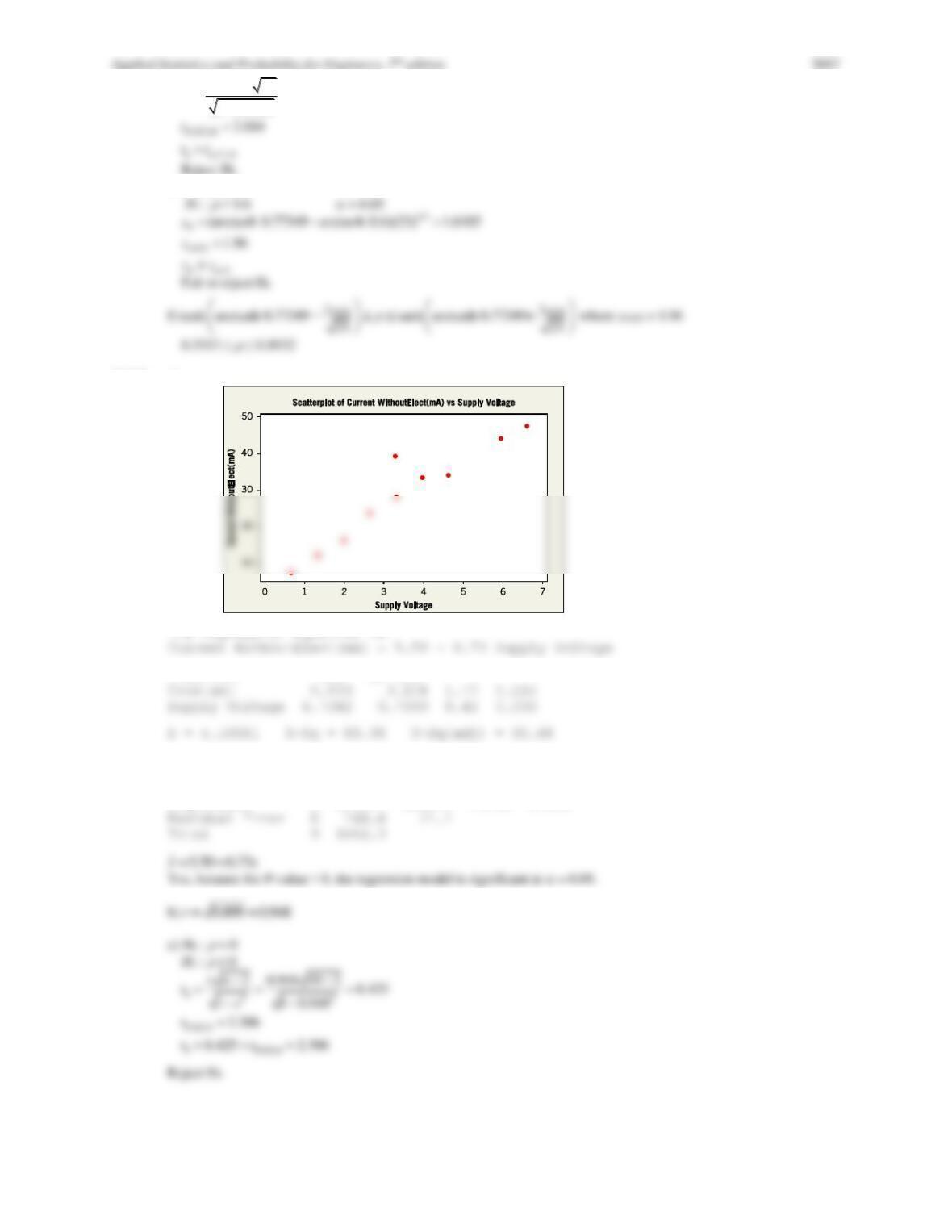
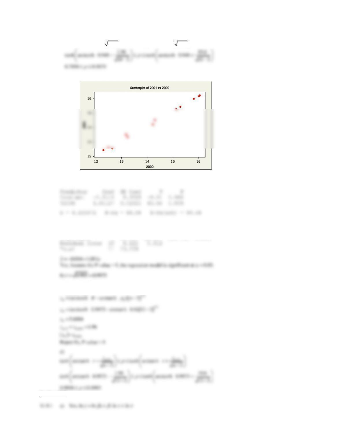
11.8.6 a)
The regression equation is
Y2001 = – 0.014 + 1.01 Y2000
Analysis of Variance
Source DF SS MS F P
Regression 1 23.117 23.117 1897.63 0.000
c) H0 :
= 0.9
H1 :
≠ 0.9
Section 11-9
Applied Statistics and Probability for Engineers, 7th edition 2017
11-29
yx
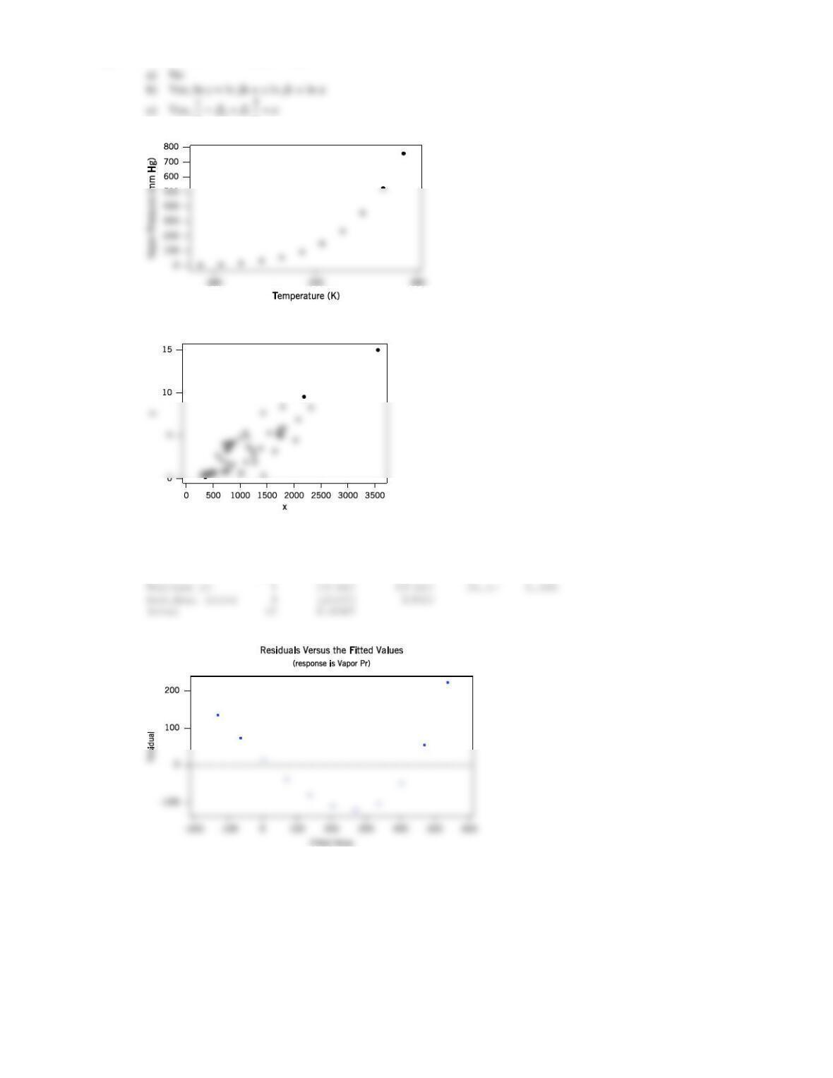
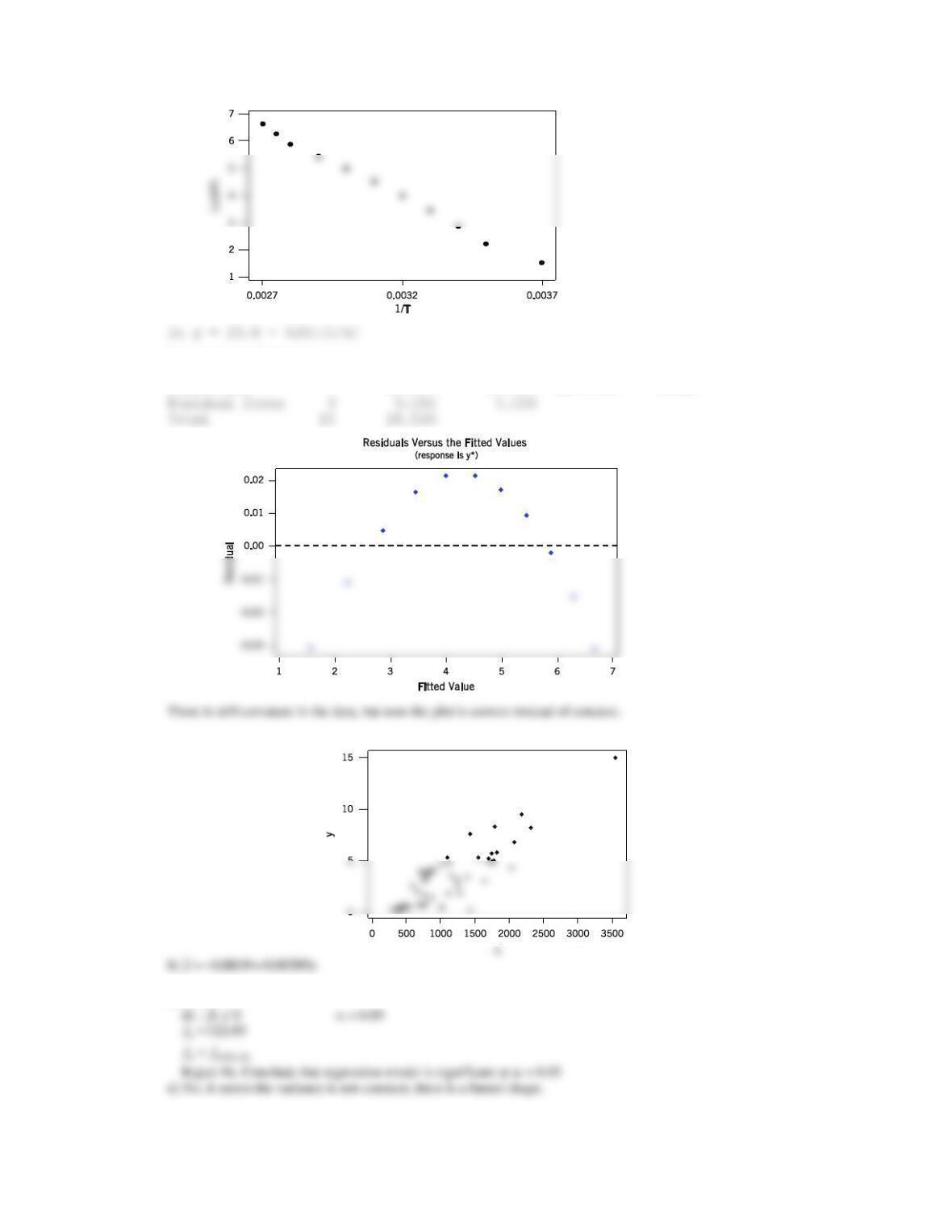
11.9.2 a) There is curvature in the data.
b) y = – 1956.3 + 6.686 x
c)
Source DF SS MS F P
d)
There is curvature in the plot of the residuals.
Applied Statistics and Probability for Engineers, 7th edition 2017
11-30
e) The data are linear after the transformation to y* = ln y and x* = 1/x.
Analysis of Variance
Source DF SS MS F P
Regression 1 28.511 28.511 66715.47 0.000
11.9.3 a)
c) H0 :
1 = 0
Applied Statistics and Probability for Engineers, 7th edition 2017
11-31
Section 11-10
11.10.1 a) The fitted logistic regression model is
1
ˆ
1 exp[ ( 8.73951 0.00020 )]
yx
=+ − − −
The computer results are shown below.
Binary Logistic Regression: Home Ownership Status versus Income
Link Function: Logit
Response Information
Variable Value Count
11.10.2 a) The fitted logistic regression model is
1
ˆ
1 exp[ (5.33971 0.00155 )]
yx
=+ − −
The computer results are shown below.
Binary Logistic Regression: Number Failing, Sample Size, versus Load, x(psi)
Link Function: Logit
Response Information
Variable Value Count