(c) Delete the two points identified in part (b) from the sample and fit the simple linear
regression model to the remaining 18 points. Calculate the value of
2
R
for the new model.
Is it larger or smaller than the value of
2
R
computed in part (a)? Why?
(d) Calculate the values of
2
ˆ
before and after the two points identified above were deleted and
the model fit to the remaining points. Did the value of
2
ˆ
change dramatically? Why?
SOLUTION
(a)
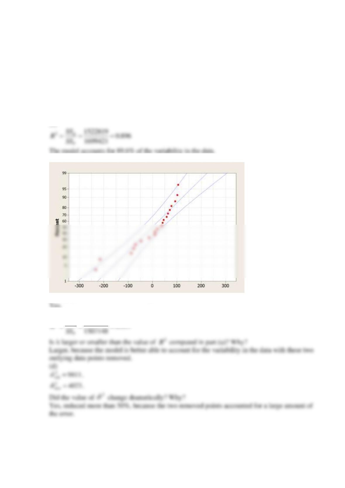
(b)
Do any points seem unusual on this plot?
(c)
2
R
21442781 0.957
R
SS
Reserve Problems Chapter 11 Section 7 Problem 8

A rocket motor is manufactured by bonding together two types of propellants, an igniter and a
sustainer. The shear strength of the bond y is thought to be a linear function of the age of the
propellant x when the motor is cast. The following table provides 20 observations. The fitted
simple regression model equation is
2625.39 36.962
ˆ
yx=−
.
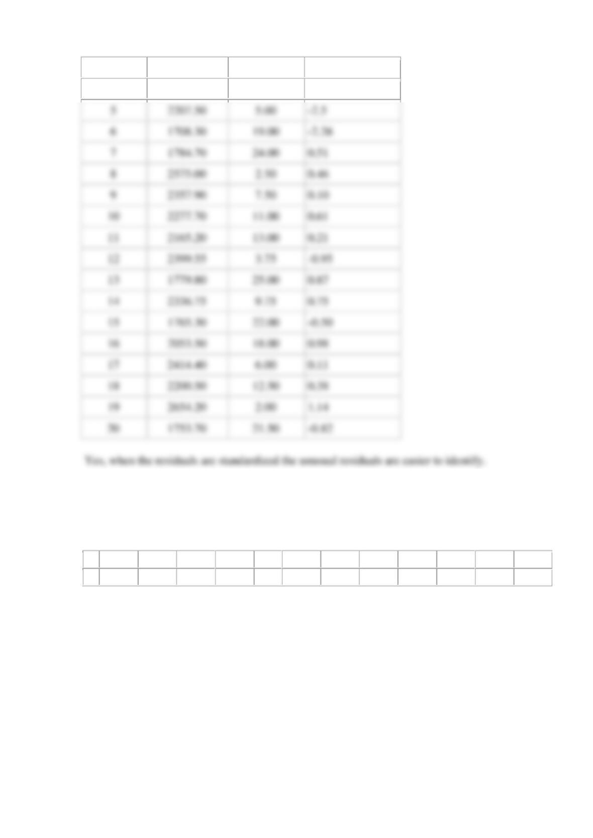
Calculate the standardized residuals for these data. Does this provide any helpful information
about the magnitude of the residuals?
Observation
number
Strength y (psi)
Age x (weeks)
Standardized error
1
2158.70
15.50
2
1678.15
23.75
3
2316.00
8.00
4
2061.30
17.00
5
2207.50
5.00
6
1708.30
19.00
7
1784.70
24.00
8
2575.00
2.50
9
2357.90
7.50
10
2277.70
11.00
11
2165.20
13.00
12
2399.55
3.75
13
1779.80
25.00
14
2336.75
9.75
15
1765.30
22.00
16
2053.50
18.00
17
2414.40
6.00
18
2200.50
12.50
19
2654.20
2.00
20
1753.70
21.50
SOLUTION
Observation
number
Strength y (psi)
Age x (weeks)
Standardized error
1
2158.70
15.50
1.10
2
1678.15
23.75
-0.76
3
2316.00
8.00
-0.14
4
2061.30
17.00
0.67
Reserve Problems Chapter 11 Section 8 Problem 1
The average daily cost of living in dollars (x) and the average wage in dollars (y) in 12 regions of
a country are shown in the following table.
x
76
83
83
84
88
105
68
90
70
88
77
115
y
132
148
135
157
16
193
135
154
154
161
156
172
Assume that the averages are jointly normally distributed.
(a) Find a regression line relating the wage to the cost of living.
(b) Test for the significance of regression using
0.01
=
.
(c) Estimate the correlation coefficient.
5
2207.50
5.00
-2.5
6
1708.30
19.00
-2.26
7
1784.70
24.00
0.51
8
2575.00
2.50
0.46
9
2357.90
7.50
0.10
2277.70
11.00
0.61
2165.20
13.00
0.21
2399.55
3.75
-0.95
1779.80
25.00
0.87
2336.75
9.75
0.75
1765.30
22.00
-0.50
2053.50
18.00
0.98
2414.40
6.00
0.11
2200.50
12.50
0.38
2654.20
2.00
1.14
1753.70
21.50
-0.82
(d) Test the hypothesis that
0
=
, using
0.01
=
.
(e) Test the hypothesis that
0.4
=
, using
0.05
=
.
(f) Construct a 95% confidence interval for the correlation coefficient.
SOLUTION
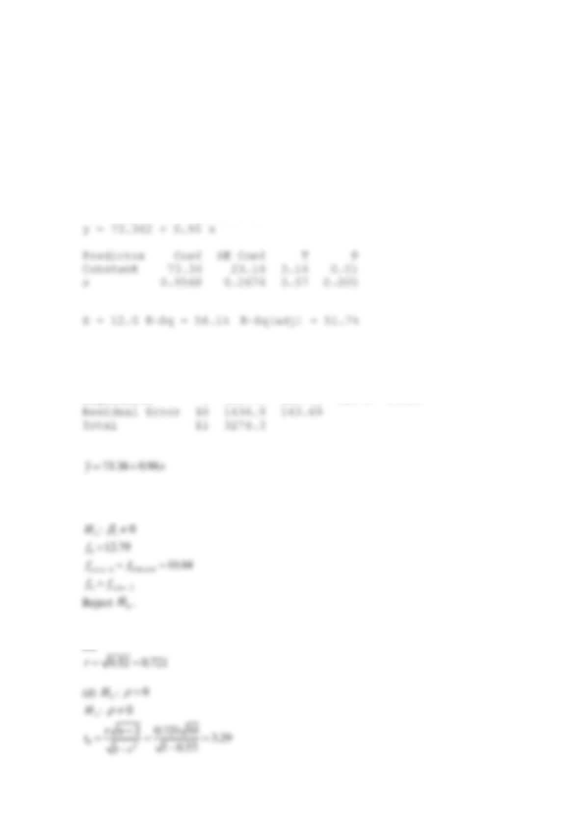
(a)
The regression equation is
Analysis of Variance
Source
DF
SS
MS
F
P
Regression
1
1837.3
1837.3
12.79
0.005
10
1436.9
143.69
Total
11
3274.3
(b)
0
H
:
10
=
0
H
0
=
Predictor
P
Constant
3.16
0.9568
3.57
0.005
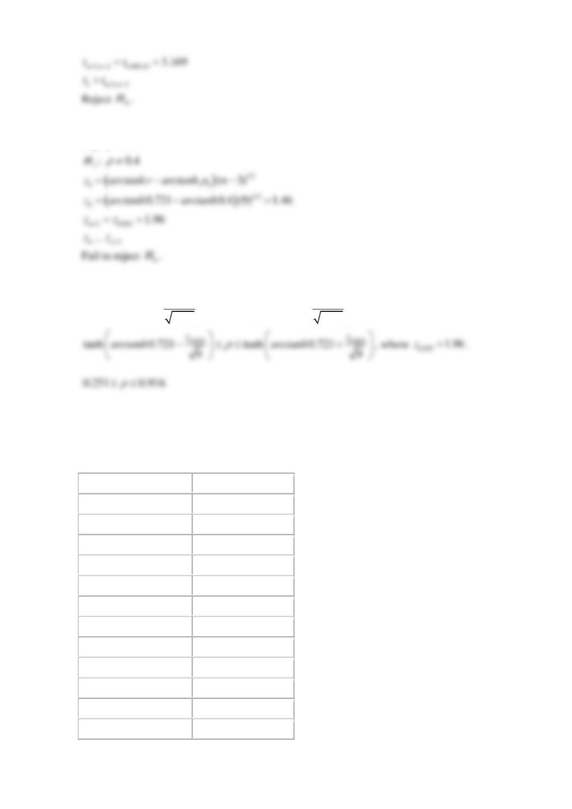
(e)
H
:
0.4
=
(f)
/2 /2
tanh tanh
33
zz
arctanh r arctanh r
nn
− +
−−
Reserve Problems Chapter 11 Section 8 Problem 2
The following table contains the average number of employees per 100 hectares (x) and the
production rate per 100 hectares (y) at 15 different farms in a region.
x
y
8.1
413
15.9
701
10.5
506
6.8
380
9.6
454
12.2
487
9.2
399
10.4
493
7.6
310
4.7
277
6.1
290
12.2
592
H
17.4
707
14.1
555
6.2
237
Assume that the averages are jointly normally distributed.
(a) Find a regression line relating the production rate to the number of employees.
(b) Test for the significance of regression using
0.01
=
.
(c) Estimate the correlation coefficient.
(d) Test the hypothesis that
0
=
, using
0.05
=
.
(e) Test the hypothesis that
0.7
=
, using
0.01
=
.
(f) Construct a 90% confidence interval for the correlation coefficient.
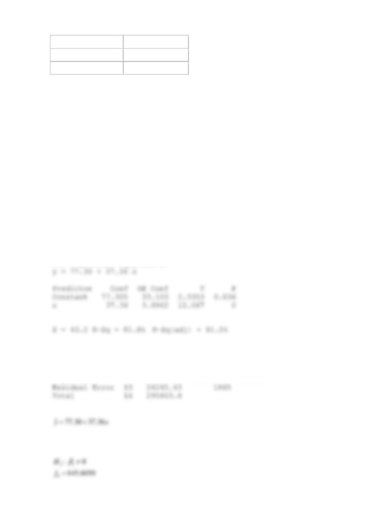
SOLUTION
(a)
The regression equation is
Analysis of Variance
Source
DF
SS
MS
F
P
Regression
1
271558.16
271558.16
145.60
0
13
Total
14
(b)
0
H
:
10
=
Predictor
T
Constant
77.305
2.3353
0.036
12.067
(c)
(d)
0
H
:
0
=
1
H
0
0
H
(e)
0
H
:
0.7
=
1
H
:
0.7
0
H
(f)
/2 /2
tanh tanh
33
zz
arctanh r arctanh r
nn
− +
−−
Reserve Problems Chapter 11 Section 8 Problem 3
Suppose that data are obtained from 50 pairs of
( )
,xy
and the sample correlation coefficient is
0.58.
(a) Test the hypothesis
0
H
:
0
=
against
1
H
:
0
with
0.01
=
. Calculate the P-value.
(b) Test the hypothesis
0
H
:
0.7
=
against
1
H
:
0.7
with
0.01
=
. Calculate the P-value.
0
H
(c) Construct a 90% two-sided confidence interval for the correlation coefficient.
SOLUTION
(a)
0
H
:
0
=
(b)
0
H
:
0.5
=
1
H
:
0.5
0
H
(c)
/2 /2
tanh tanh
33
zz
arctanh r arctanh r
nn
− +
−−
Reserve Problems Chapter 11 Section 8 Problem 4
A random sample of 50 observations was made on the diameter of spot welds and the
corresponding weld shear strength.
(a) Given that
0.62r=
, test the hypothesis that
0
=
, using
0.01
=
.
(b) Find a 99% confidence interval for
P
.
(c) Based on the confidence interval in part (b), can you conclude that
0.5PI =
at the 0.01 level
of significance?
0
H
SOLUTION
(a)
( )
022
2 0.62 48 5.47
11 0.62
rn
t
r
−
= = =
−−
(b)
(c)
Reserve Problems Chapter 11 Section 9 Problem 1
The following table represents water density at different temperatures.
x (temperature, °C)
y (density, kg/m3)
0
999.9
5
1000.0
10
999.7
20
998.2
30
995.7
40
992.2
50
988.1
60
983.2
70
977.8
80
971.8
90
965.3
100
958.4
(a) Draw a scatter diagram of these data. Does the linear regression model seem adequate?
(b) Draw a scatter diagram using
2
xx
=
as a variable. Does this transformation seem
appropriate for linearization?
SOLUTION
(a)
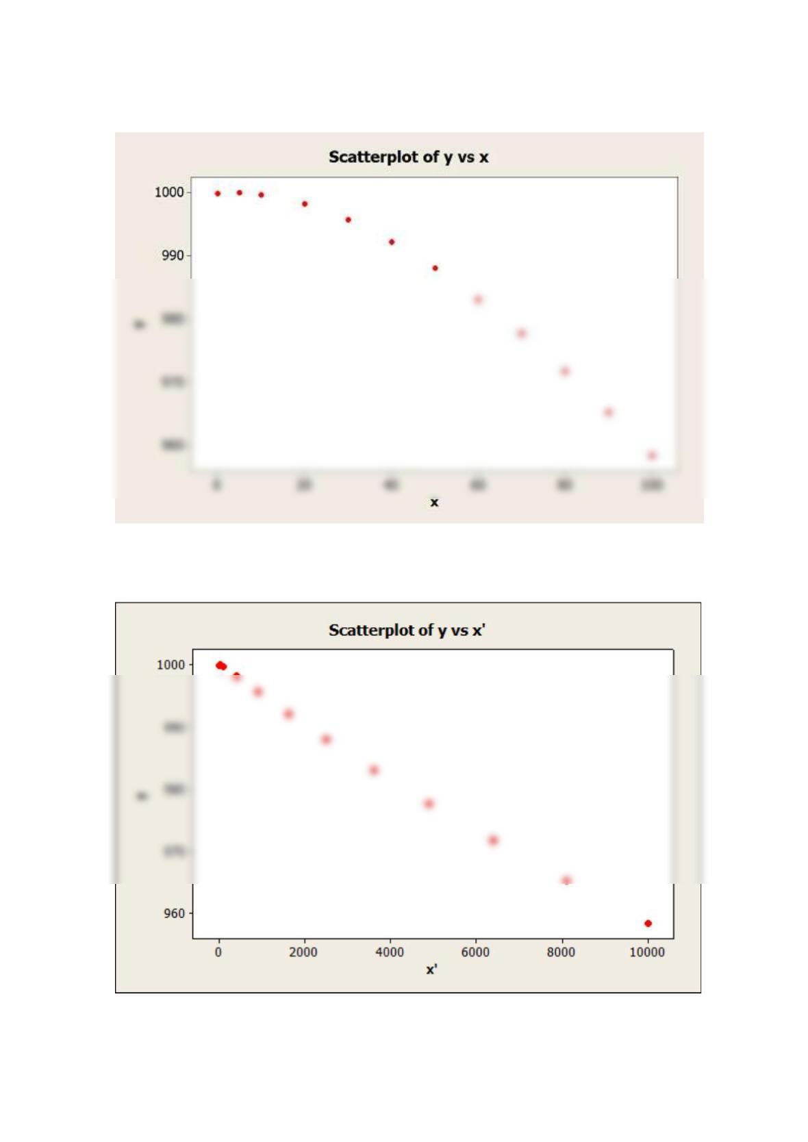
The scatter diagram below exhibits a nonlinear relationship between x and y. Therefore, the
linear regression model does not seem adequate.
(b)
The data seem to be linear after the transformation
2
xx
=
, indicating that this transformation is
appropriate for linearization.
Reserve Problems Chapter 11 Section 10 Problem 1

In 2008, a study was conducted attempting to relate car ownership to the household income in
the Czech Republic. The income was differentiated by 10 deciles and the number of car owners
for each income decile were recorded. The complete test data are shown in the table below:
Sample size
Number of car owners
decile 1
100
54
decile 2
100
51
decile 3
100
55
decile 4
100
58
decile 5
100
54
decile 6
100
61
decile 7
100
66
decile 8
100
67
decile 9
100
68
decile 10
100
71
(a) Fit a logistic regression model to the data. Use a simple linear regression model as the
structure for the linear predictor.
(b) Is the logistic regression model in part (a) adequate?
SOLUTION
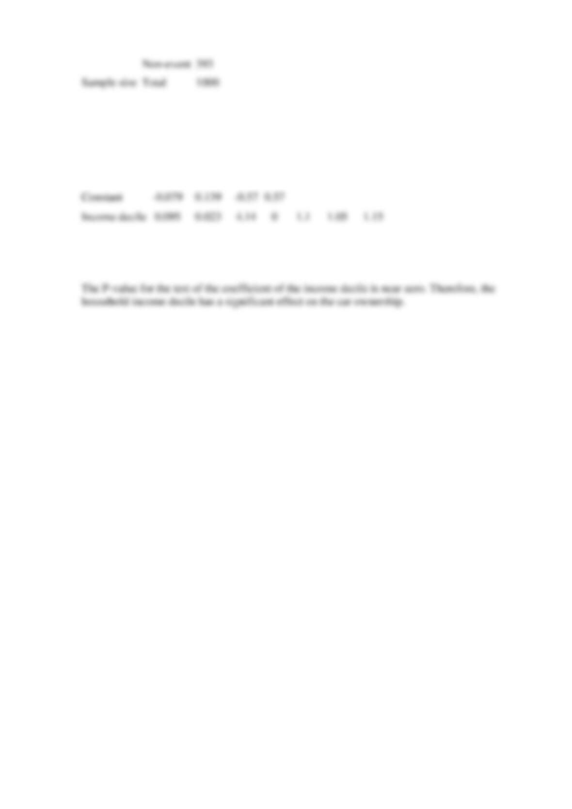
(a)
The fitted logistic regression model is
Binary Logistic Regression: Car owners; Sample size versus Income decile
Link Function: Logit
Response Information
Logistic Regression Table
Odds
95% CI
Predictor
Coef
SE Coef
Z
P
Ratio
Lower
Upper
Constant
-0.079
-0.57
0.57
Income decile
0.095
4.14
0
(b)
Reserve Problems Chapter 11 Section 10 Problem 2
Consider the history of weather observations for the New York Airport (JFK) for April, 2017.
Assume that the absence of rain is considered a failure. Relate the average humidity to the
probability of rain with a logistic regression model.
Date
Average humidity, %
Rain Status
1
80
0
2
47
0
3
62
1
4
91
1
5
82
1
6
88
1
7
67
1
8
45
0
9
53
0
10
71
1
11
80
0
12
73
0
13
46
0
14
58
0
15
75
1
16
71
1
17
55
0
Non-event
393
Sample size
Total
1000
18
59
0
19
76
1
20
84
1
21
90
1
22
79
1
23
68
0
24
77
1
25
93
1
26
92
1
27
92
1
28
81
0
29
72
1
30
66
0
(a) Fit a logistic regression model to the response variable y (
1y=
indicates that it rained and
0y=
indicates that it did not rain). Use a simple linear regression model as the structure for the
linear predictor.
(b) Is the logistic regression model in part (a) adequate?
(c) Provide an interpretation of the parameter
1
in this model.
(d) What is the estimated probability of the rain when the average humidity is 85%?
SOLUTION
(a)
The fitted logistic regression model is
Binary Logistic Regression: Rain Status versus Average humidity
Link Function: Logit
Response Information
Logistic Regression Table
Odds
95% CI
Predictor
Coef
SE Coef
P
Ratio
Lower
Upper
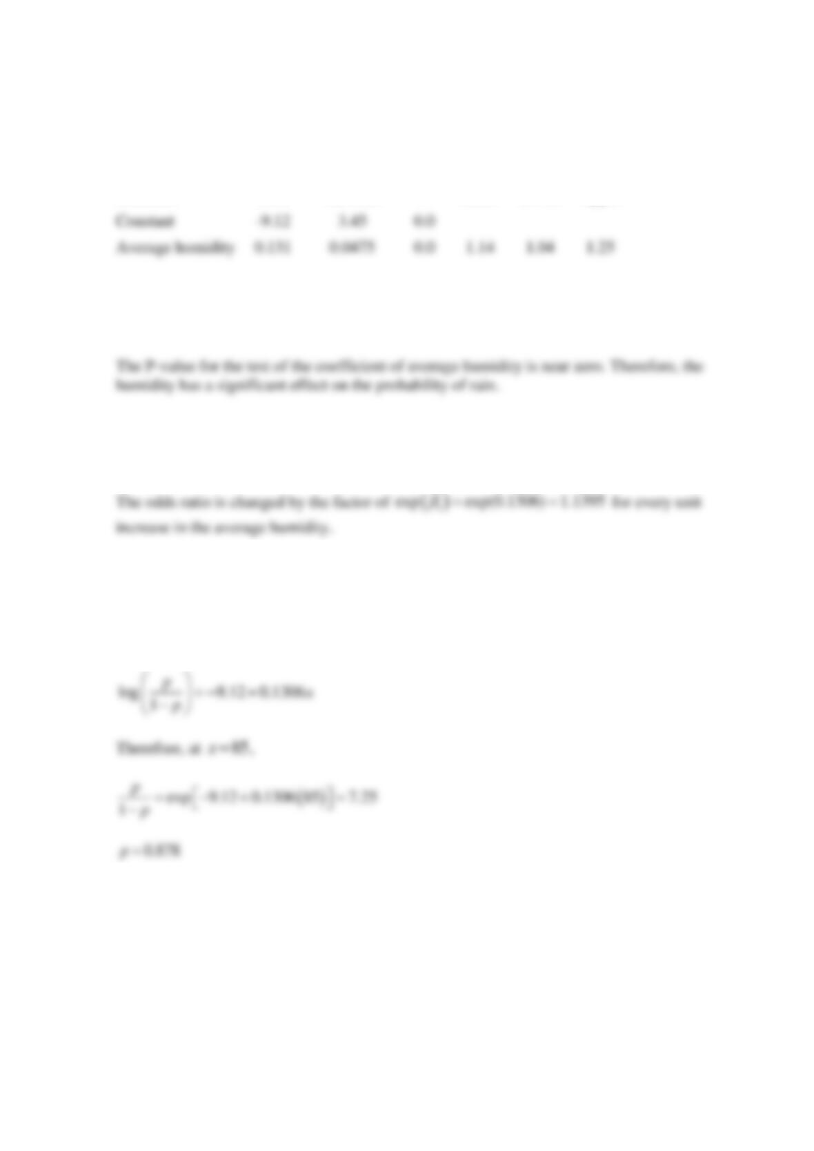
(b)
(c)
(d)
The fitted model is
Reserve Problems Chapter 11 Section 10 Problem 3
A study was conducted attempting to relate the number of days before the rock-concert and the
probability that it is still possible to buy a ticket. Assume that the absence of tickets is considered
a failure. The obtained data are shown in the table below:
Days before concert
Availability of tickets
180
1
Constant
-9.12
0.0
Average humidity
0.0
1.04
178
1
132
1
132
1
120
1
81
1
74
1
65
1
60
0
56
0
49
0
42
0
39
0
30
0
25
0
21
0
15
0
10
0
7
1
4
0
1
0
(a) Fit a logistic regression model to the response variable y (
1y=
indicates that there are
available tickets and
0y=
indicates the sold-out). Use a simple linear regression model as the
structure for the linear predictor.
(b) Is the logistic regression model in part (a) adequate?
(c) Provide an interpretation of the parameter
1
in this model.
(d) What is the estimated probability that it is possible to buy a ticket if there are 90 days left
before the concert?
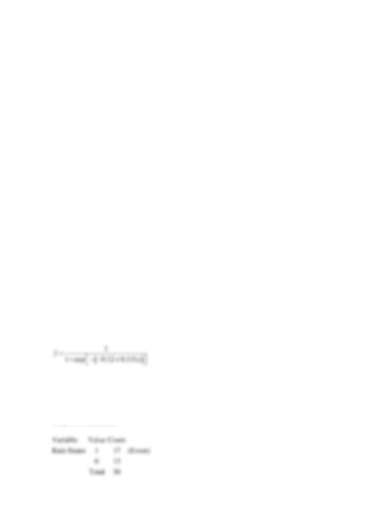
SOLUTION
(a)
The fitted logistic regression model is
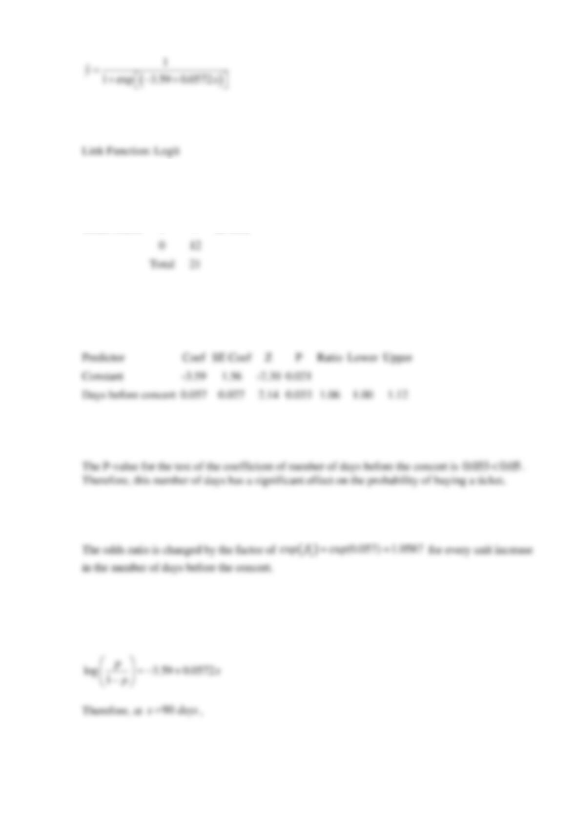
Binary Logistic Regression: Ticket status versus Days before concert
Response Information
Variable
Value
Count
Ticket Status
1
9
(Event)
0
Logistic Regression Table
Odds
95% CI
Predictor
SE Coef
Ratio
Lower
Upper
Constant
-2.30
0.021
Days before concert
0.057
0.033
(b)
(c)
(d)
The fitted model is

Reserve Problems Chapter 11 Section 10 Problem 4
Consider the situation when a foundation of charitable scholarships initiates an open-access
contest in order to distribute the scholarships for the current term. The survey was conducted
among the students of different departments in order to determine the relationship between GPA
(on a ten-point scale) and the probability of gaining the scholarship. The obtained data are shown
in the table below:
GPA
Scholarship status
11.0
1
10.5
1
8.8
1
8.7
0
8.4
1
8.2
0
8.1
0
7.9
1
7.8
0
7.7
1
7.4
0
7.3
0
7.2
0
7.0
0
(a) Fit a logistic regression model to the response variable y (
1y=
indicates that a student gains
the scholarship and
0y=
indicates that he/she does not). Use a simple linear regression model
as the structure for the linear predictor.
(b) Is the logistic regression model in part (a) adequate?
(c) What is the estimated probability to gain a scholarship if GPA equals 8.0?
SOLUTION
(a)
The fitted logistic regression model is
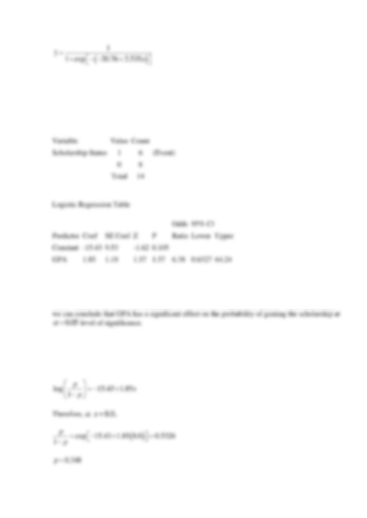
Binary Logistic Regression: Scholarship status versus GPA
Link Function: Logit
Response Information
(b)
The P-value for the test of the coefficient of GPA is 0.048 that is less than
0.05
=
. Therefore,
(c)
The fitted model is

Reserve Problems Chapter 11 Section 10 Problem 5
The weight and systolic blood pressure of 26 randomly selected males in the age group 25 to 30
are shown in the following table. Assume that weight and blood pressure are jointly normally
distributed.
Weight (x)
Systolic BP (y)
165
130
167
133
180
150
155
128
212
151
175
146
190
150
210
140
200
148
149
125
158
133
169
135
170
150
172
153
159
128
168
132
174
149
183
158
215
150
195
163
180
156
143
124
240
170
235
165
192
160
187
159
Fit a no-intercept model to the data.
SOLUTION
Reserve Problems Chapter 11 Section 10 Problem 6
The grams of solids removed from a material (y) is thought to be related to the drying time. Ten
observations obtained from an experimental study follow:
y
4.3
1.5
1.8
4.9
4.2
4.8
5.8
6.2
7.0
7.9
x
2.5
3.0
3.5
4.0
4.5
5.0
5.5
6.0
6.5
7.0
(a) Fit a simple linear regression model for these data.
(b) Test for significance of regression.
(c) Based on these data, what is your estimate of the mean grams of solid removed at 4.25 hours?
Find a 95% confidence interval on the mean.
SOLUTION
(a)