Unlock document.
This document is partially blurred.
Unlock all pages and 1 million more documents.
Get Access
1
Solutions To Problems of Chapter 4
4.1. Show that the set of equations
Σθ=p
has a unique solution if Σ > 0 and infinite many if Σis singular.
Solution: a) Let Σ > 0. Then the linear system of equations has a unique
solution. The converse is also true. Let the linear system has a unique
4.2. Show that the set of equations
Σθ=p
has always a solution.
Solution: The existence of solution when Σ > 0 is obvious. Let Σbe singu-
lar. Then, in order to guarantee a solution, we have to show that plies in
the range space of Σ. For this, it suffices to show that p⊥a,∀a∈ N (Σ).
2
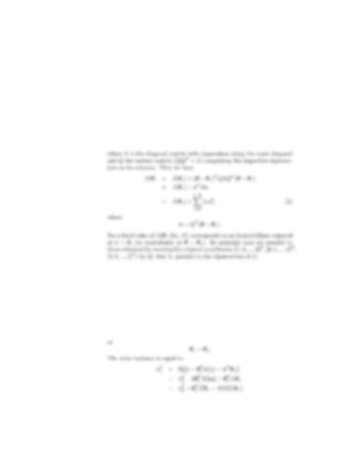
4.3. Show that the shape of the isovalue contours of the mean-square error
(J(θ)) surface,
J(θ) = J(θ∗)+(θ−θ∗)TΣ(θ−θ∗),
are ellipses whose axes depend on the eigenstructure of Σ.
Hint: Assume that Σhas discrete eigenvalues.
Solution: Since Σis symmetric, we know that it can be diagonalized,
Σ=QΛQT,
4.4. Prove that if the true relation between the input xand the true output y
is linear, i.e.,
y = θT
ox+ v,θo∈Rl
where v is independent of x, then the optimal MSE θ∗satisfies
θ∗=θo.
Solution: The optimal parameter vector is given by
Σθ∗=E[xy] = E[xxTθo+ v]
=Σθo,
3
4.5. Show that if
y = θT
ox+ v,θo∈Rk
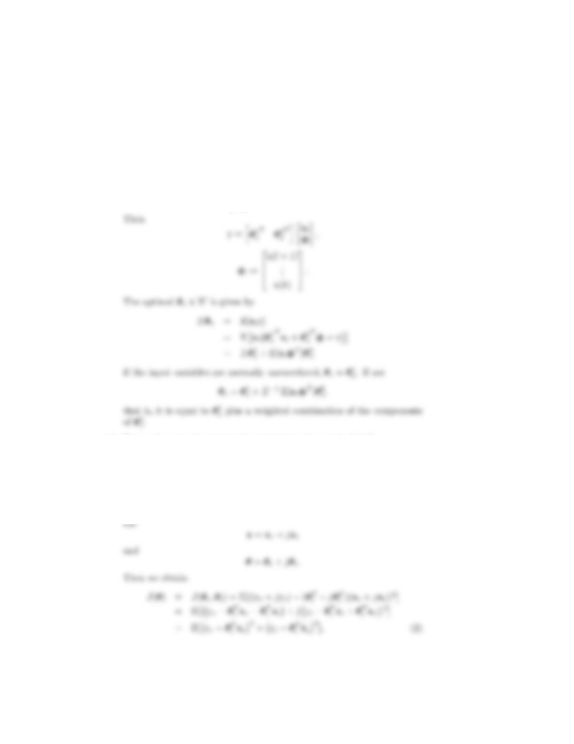
where v is independent of x, then the optimal MSE θ∗∈Rl, l < k is equal
to the top lcomponents of θo, if the components of xare uncorrelated.
Solution: Let
θo=θ1
o
θ2
o,θ1
o∈Rl,θ2
o∈Rk−l.
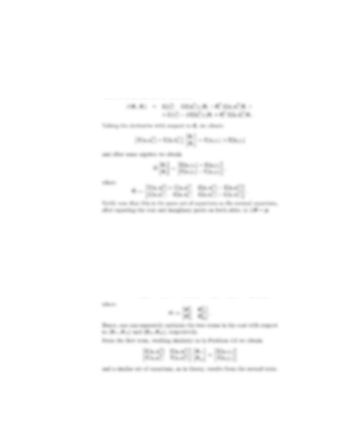
4.6. Derive the normal equations by minimizing the cost in (4.15).
Hint: Express the cost in terms of the real part θrand its imaginary part
θiof θand optimize with respect to θr,θi.
Solution: The cost function is
J(θ) := E|y−θHx|2.
4
where
θ=θr
θi,x=xr
xi,˜
x=xi
−xr.(3)
The cost in (2) can now be written as
4.7. Consider the multichannel filtering task
ˆ
y=ˆyr
ˆyi= Θ xr
xi.
Estimate Θ so that to minimize the error norm:
E[||y−ˆ
y||2].
Solution: The error norm is equal to
J(Θ) = Eyr−ˆyr2+Eyi−ˆyi2
=Eyr−θT
11xr−θT
12xi2+Eyi−θT
21xr−θT
22xi2,
5
4.8. Show that (4.34) is the same as (4.25).
Solution: By the respective definitions, we have
ˆyr+jˆyi= (θT
r−jθT
i)(xr+jxi) +
4.9. Show that the MSE achieved by a linear complex-valued estimator is al-
ways larger than that obtained by a widely linear one. Equality is achieved
only under the circularity conditions.
Solution: The minimum MSE for the linear filter is
MSEl=E[(y −θH
∗x)(y∗−xHθ∗)]
=E[y2] + θH
∗E[xxH]θ∗−θH
∗E[xy∗]−E[yxH]θ∗

6
4.10. Show that under the second order circularity assumption, the conditions
in (4.39) hold true.
Solution: By the second order circularity condition we have
E[xxT]=0,
4.11. Show that if
f:C−→ R,
then the Cauchy-Riemann conditions are violated.
Proof: Let
f(x+jy) = u(x, y)∈R.
Then by assumption, the imaginary part v(x, y) is identically zero. Hence
the Cauchy-Riemann conditions, i.e.,
4.12. Derive the optimality condition in (4.45).
Solution: We will show that any other filter, hi, i ∈Z, results in a larger
MSE compared to the filter wi, i ∈Z, which satisfies the condition. In-
deed, we have that
A:= E(dn−X
i
hiun−i)2=E(dn−X
i
(hi−wi+wi)un−i)2.
j
i
7
4.13. Show Equations (4.50) and (4.51).
Solution:
a) Eq. (4.51): We know from Chapter 2 that the power spectrum of the
output process, y(n, m) is related to that of the input, d(n, m), by
b) Eq. (4.50): By the respective definition we have that,
rdu(k, l) = Ed(n, m)u(n−k, m −l),
and also
+∞
X
+∞
X
i0=−∞
j0=−∞

8
4.14. Derive the normal equations for Example 4.2.
Solution: We have
E[unun] = E0.5sn+ sn−1+ηn0.5sn+ sn−1
+ηn
= 0.25rs(0) + rs(0) + rη(0)
Similarly,
E[undn] = Eunsn−1
4.15. The input to the channel is a white noise sequence snof variance σ2
s. The
output of the channel is the AR processes
yn=a1yn−1+ sn.(5)
The channel also adds white noise ηnof variance σ2
η. Design an optimal
equalizer of order two, which at its output recovers an approximation of
sn−L. Sometimes, this equalization task is also known as whitening, since
in this case the action of the equalizer is to “whiten” the AR process.
Solution: The input to the equalizer is
un= yn+ηn.
9
Thus, the elements of the input covariance/autocorrelation matrix are
given by
•ru(0) = E[unun] = E[(yn+ηn)(yn+ηn)]
s
1−a2
1
1−a2
1
η
4.16. Show that the forward and backward MSE optimal predictors are conju-
gate reverse of each other.
Solution: By the respective definitions we have
am=Σ−1
mr∗
m
10
Since Σmis a Hermitian Toeplitz matrix, it is easily checked out that
4.17. Show that the MSE prediction errors (αf
m=αb
m) are updated according
to the recursion
αb
m=αb
m−1(1 − |κm−1|2).
Solution: By the respective definition we have
αb
m=r(0) −rH
mJmΣ−1
mJmrm=r(0) −rH
mJmbm=r(0) −rH
ma∗
m
=r(0) −rH
m−1r∗(m)(a∗
m−1
0+−b∗
m−1
1κ∗
m−1)
4.18. Derive the BLUE in the Gauss-Markov theorem.
Solution: The optimization task is
H∗:= arg minHtrace{HΣηHT},
.
.
hT
l
11
Observe that
trace{HΣηHT}=
l
X
i=1
hT
iΣηhi.(6)

12
4.19. Show that the mean-square error (which in this case coincides with the
variance of the estimator) of any linear unbiased estimator is higher than
that associated with the BLUE.
Solution: The mean-square error of any His given by
MSE(H) = trace{HΣηHT}.
However,
Hence,
HΣηHT
∗=HΣηΣ−1
ηX(XTΣ−1
ηX)−1= (XTΣ−1
ηX)−1.
13
4.20. Show that if Σηis positive definite, then XTΣ−1
ηXis also positive definite
if Xis full rank.
Solution: Recall from linear algebra that if Xis full rank, then XTX
is positive definite and vice versa. Indeed, assume that this is not the
case. Then, there will be a6=0, such that
XTXa=0,
4.21. Derive a MSE optimal linearly constrained widely linear beamformer.
Solution: The output of the widely linear beamformer is given by
ˆs(t) = wHu(t) + vHu∗(t)
14
The error signal is
Let us write the two constraints in a more compact form to facilitate the
optimization. To this end, we have that
XH˜
we=1
0,
where

15
and finally
4.22. Prove that the Kalman gain that minimizes the error variance matrix
Pn|n=E[(xn−ˆ
xn|n)(xn−ˆ
xn|n)T],
is given by
Kn=Pn|n−1HH
n(Rn+HnPn|n−1HT
n)−1.
Hint: Use the following formulas
∂trace{AB}
∂A =BT(AB a square matrix)
∂trace{ACAT}
∂A = 2AC, (C=CT).
Solution: We know that
ˆ
xn|n=ˆ
xn|n−1+Kn(yn−Hnˆ
xn|n−1).
Thus,
Pn|n=E(xn−ˆ
xn|n)(xn−ˆ
xn|n)T
16
Hence, we have that
4.23. Show that in Kalman filtering, the prior and posterior error covariance
matrices are related as
Pn|n=Pn|n−1−KnHnPn|n−1.
which results in the desired update.
4.24. Derive the Kalman algorithm in terms of the inverse state-error covariance
matrices, P−1
n|n. In statistics, the inverse error covariance matrix is related
to Fisher’s information matrix, hence the name of the scheme.
Solution: To build the Kalman algorithm around the inverse state-error
covariance matrices P−1
n|n, P −1
n|n−1, we need to apply the following matrix
inversion Lemmas,

17
which gives


