Angel and Shreiner: Interactive Computer Graphics, Seventh
Edition
Chapter 11 Solutions
11.1 (m+ 1)3
11.2 The function y=f(x) describes the same curve in any plane of
constant z, or equivalently, a curve in the y, z plane that is extruded in z
to form a surface. Likewise the function z=g(x) describes a surface
11.3 As uvaries over (a, b), v=u−a
b−avaries over (0,1). Substituting into
the polynomial p(u) = Pn
11.4 The interpolating matrix for interpolating points x0,x1,x2and x3is
A=
1x0x2
0x3
0
1x1x2
1x3
1
1x2x2
2x3
2
1x3x2
3x3
3
.
11.5 Consider the Bernstein polynomial
bkd(u) = d
k!uk(1 −u)d−k.
For k= 0 or k=d, the maximum value of 1 is at one end of the interval
(0,1) and the minimum is at the other because all the zeros are at 1 or 0.
1
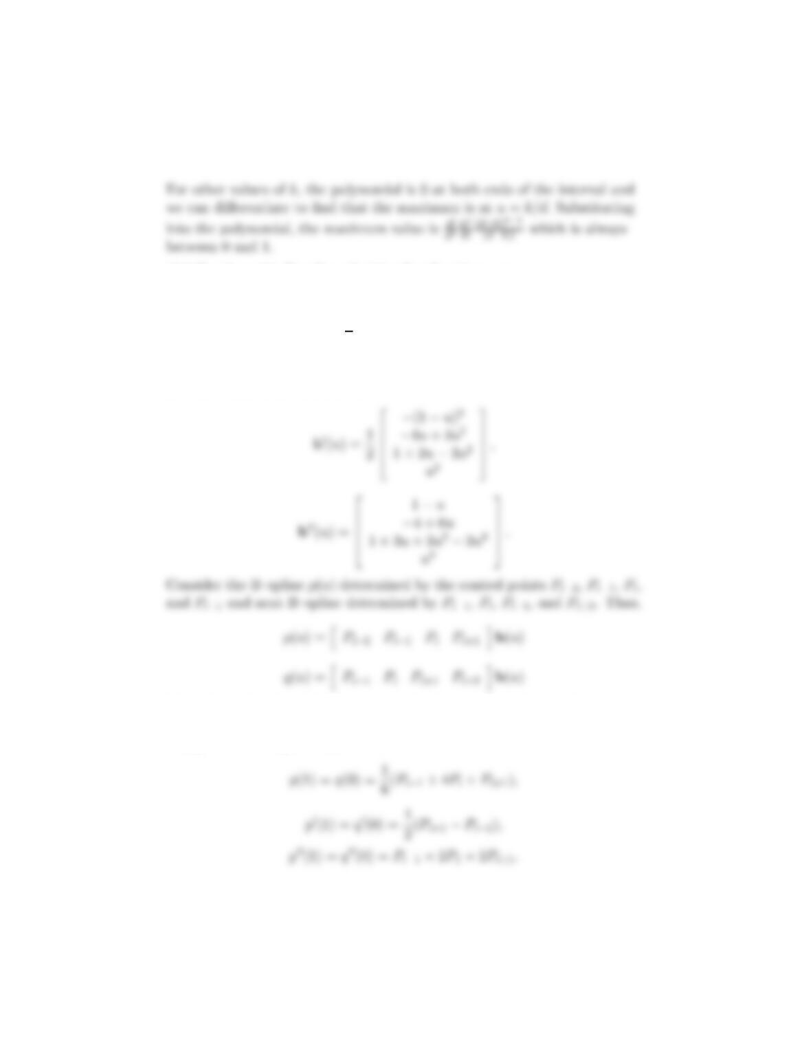
11.6 For the cubic B–spline, the blending functions are
b(u) = 1
6
(1 −u)3
4−6u2+ 3u3
1 + 3u+ 3u2−3u3
u3
,
and the first two derivatives are
−(1 −u)2
−4u+ 3u2
The values of p(u) and its first two derivatives at u= 1 have to be
compared with the values of q(u) and its first two derivatives ar u= 0.
Using the above equations, we find
2
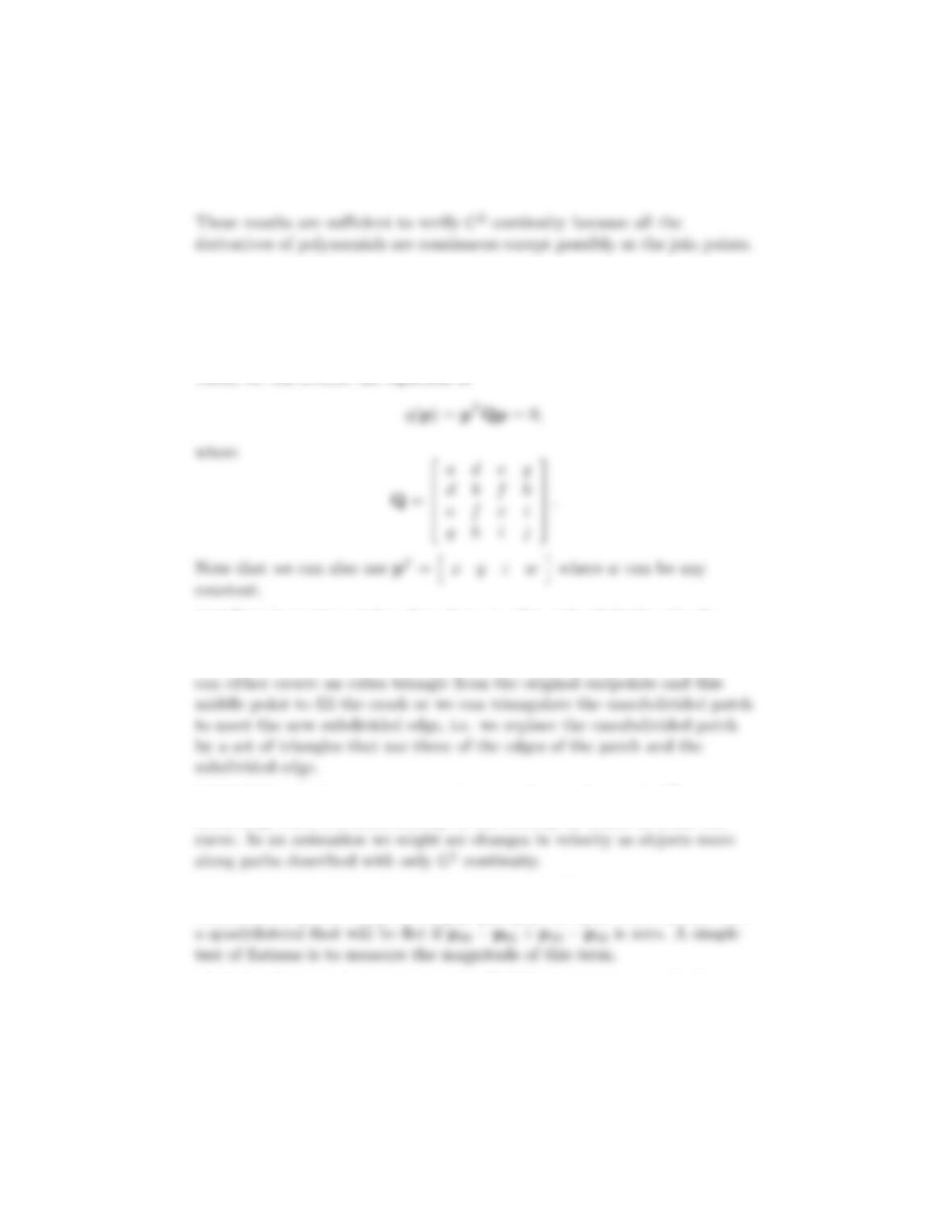
11.7 Any quadric can be written as
q(x, y, z) = ax2+by2+cz2+ 2dxy + 2exz + 2fyz + 2gx + 2hy + 2iz +j= 0,
where a, b, c, d, e, f, g, h, i and jare constants. Let pT=hx y z 1i.
Then, we can rewrite the equation as
11.8 If we have two patches that share an edge and subdivide only the
patch on one side of this edge, we can create a crack. The middle shared
endpoint on the subdivided patch does not have to lie on original edge. We
11.10 Although the curves are continuous, when we have only G1
continuity, there is a discontinuity in the velocity at which we trace the
11.12 One simple test is to use the twist (page 590). Suppose that the four
corners of the patch are given by p00,p01,p10, and p11. These points form
11.14 For the given knot sequence, the B–Spline becomes a quadratic
Bezier curve in the interval (0,1) and the three blending functions are u2,
3
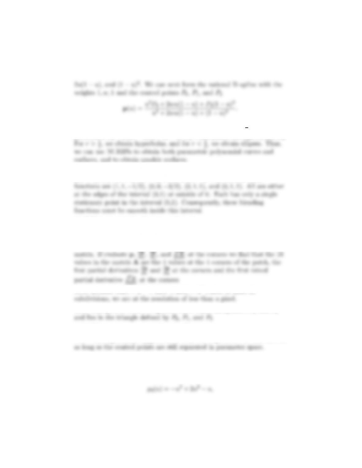
11.15 For r= 0 we get the line between P0and P2. For r=1
2we get the
parabola u2P0+ 2u(1 −u)P1+ (1 −u)2P2which passes through P0and P2.
11.16 The four blending functions for the Hermite curve are (u−1)2,
(2u+ 1), u2(−2u+ 3, u(1 −u)2, and u2(u−1). The zeros of these
11.17 We can write the Hermite surface as
p(u, v) = uTMHQMT
Hv=uTAv,
where Qcontains the control point data and MHis the Hermite geometry
11.18 Because 1024 = 210 <1280 <2048 = 211, after at most 11
11.19 This process creates a quadric curve which interpolates P0and P2
11.20 This process generates the cubic Bezier curve.
11.21 Nothing unusual happens other than the slope at u= 0 must be zero
11.22 CAD, Animation, Car and airplane design.
11.25 The columns of the matrix MRcontain the coefficients of the
blending polynomials which are
4
11.26 The required matrix is
6 12 −6 1
5