11/21/2018
SITUATION
LOOKING AT EXERCISE AND MARKET VALUE OF AN OPTION
Strike) price = $25
Price of Strike Exercise
the stock Price Value
$0 $20.00 $0.00
$5 $20.00 $0.00
$25
Chapter 8. Mini Case for Financial Options and Applications in Corporate Finance
$1.00
$7.50
$12.00
$16.50
$21.00
$35.00
$40.00
$45.00
$30.00
$5.00
$2.50
$2.00
$1.50
$25.00
$3.00
$0.50
To begin, you gathered some outside materials on the subject and used these materials to draft a list of pertinent
questions that need to be answered. In fact, one possible approach to the paper is to use a question-and-answer
Assume that you have just been hired as a financial analyst by Triple Play Inc., a mid-sized California company
that specializes in creating high-fashion clothing. Since no one at Triple Play is familiar with the basics of
financial options, you have been asked to prepare a brief report that the firm’s executives could use to gain at
least a cursory understanding of the topics.
$0.00
$50.00
$3.00
$25.50
(1.) What are the corresponding exercise values and option time values?
Exercise Values
Option Time Values
Strike Price=
a. What is a financial option? What is the single most important characteristic of an option? Answer: See
Chapter Mini Case Show
Answer: See Chapter Mini Case Show
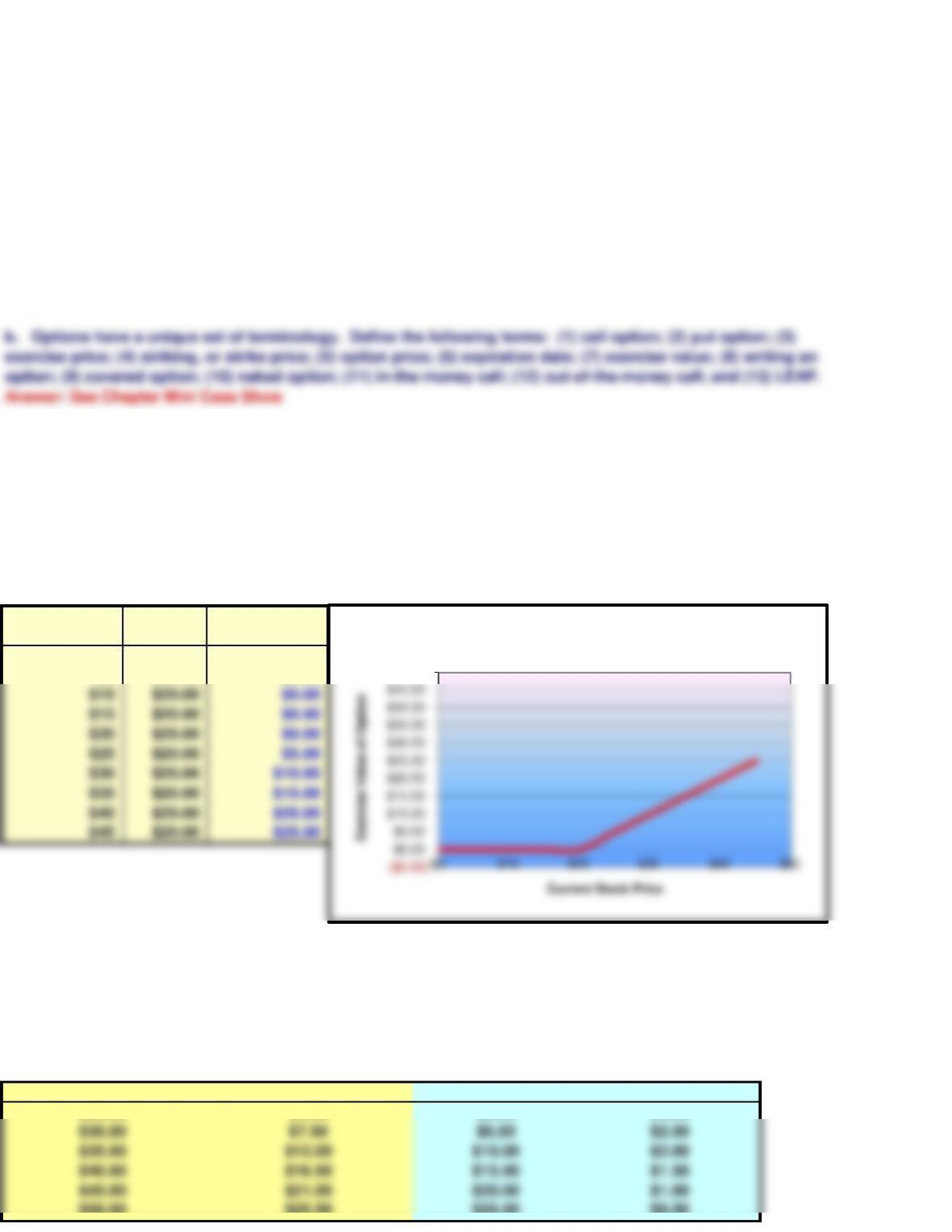
c. Consider Triple Play’s call option with a $25 strike price. The following table contains historical values for
this option at different stock prices:
Suppose a stock has the strike price shown below. The Exercise Value is the profit if you choose to exercise the
stock. If the current price of the stock is greater than the strike price, then the Exercise Value is the current stock
price minus the strike price; otherwise, it is zero (you would never exercise the option if the stock price is less
than the strike price.)
Stock Price
Option Price
$25.00
$50.00
Exercise Value vs. Stock Price
Current stock price, P = $27.00
Risk-free rate, rRF = 6%
Binomial Payoffs
Strike price: X = $25.00
Current stock price: P = $27.00
Up factor for stock price: u = 1.41
Down factor for stock price: d = 0.71
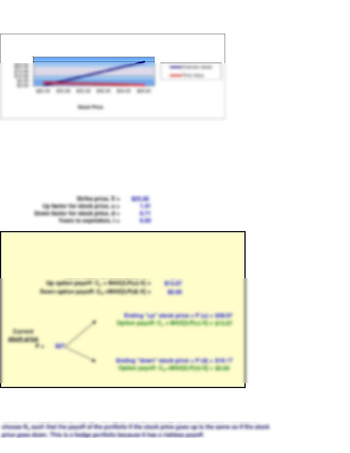
(2.) What happens to the option’s time value (the difference between the option price and its exercise value) as
the stock price rises? The time value falls as the stock price increases; see the graph below. Why? Answer: See
Chapter Mini Case Show
price goes down. This is a hedge portfolio because it has a riskless payoff.
We can form a portfolio by writing 1 call option and purchasing Ns shares of stock. We want to
d. Consider a stock with a current price of P = $27. Suppose that over the next 6 months the stock price will
either go up by a factor of 1.41 or down by a factor of 0.71. Consider a call option on the stock with a strike price
of $25 which expires in 6 months. The risk-free rate is 6%.
(1.) Using the binomial model, what are the ending values of the stock price? What are the payoffs of the call
option?
(2.) Suppose you write 1 call option and buy Ns shares of stock. How many shares must you buy to create a
portfolio with a riskless payoff (which is called a hedge portfolio)? What is the payoff of the portfolio?
$30.00
Exercise Values and Option Time Values vs. Stock Price
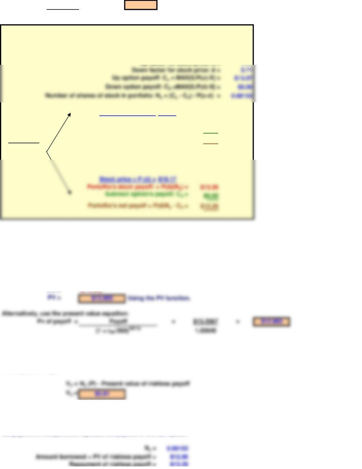
Ns = Cu – Cd=0.69153
P(u – d)
The Hedge Portfolio with Riskless Payoffs
Strike price: X = $25.00
Current stock price: P = $27.00
Up factor for stock price: u = 1.41
Stock price = P (u) = $38.07
P, Portfolio’s stock payoff: = P(u)(Ns) = $26.33
current
Subtract option’s payoff: Cu = $13.07
stock price
Portfolio’s net payoff = P(u)Ns – Cu = $13.26
$27
Stock price = P (d) = $19.17
Subtract option’s payoff: Cd = $0.00
Portoflio’s net payoff = P(d)Ns – Cd = $13.26
N = 182.5
I/YR = 0.0164%
PMT = 0
The current value of the hedge portolio is the the stock value (Ns x P) less the call value (VC). But the
hedge portfolio has a riskless payoff, so the hedge portfolio’s value must also be equal to the present
value of the riskless payoff disounted at the risk-free rate (we assume daily compounding). With a
little algebra, we get:
If you borrow an amount equal to the present value of the riskless payoff and buy Ns shares of stock,
the payoffs of this portfolio replicate the payoffs of the call option.
(4.) What is a replicating portfolio? What is arbitrage?
(3.) What is the present value of the hedge portfolio’s riskless payoff? What is the value of the call option?
The present value of the riskless payoff disounted at the risk-free rate (we assume daily
compounding) is:
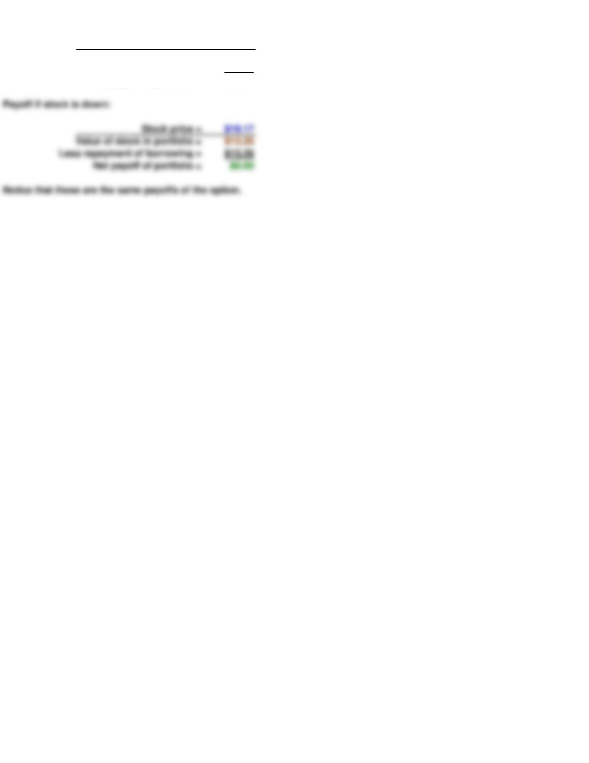
Payoff if stock is up:
Stock price = $38.07
Value of stock in portfolio = $26.33
Less repayment of borrowing = $13.26
Net payoff of portfolio = $13.07
Payoff if stock is down:
Stock price = $19.17
Value of stock in portfolio = $13.26
Less repayment of borrowing = $13.26
Net payoff of portfolio = $0.00
Notice that these are the same payoffs of the option.
BLACK-SCHOLES OPTION PRICING MODEL
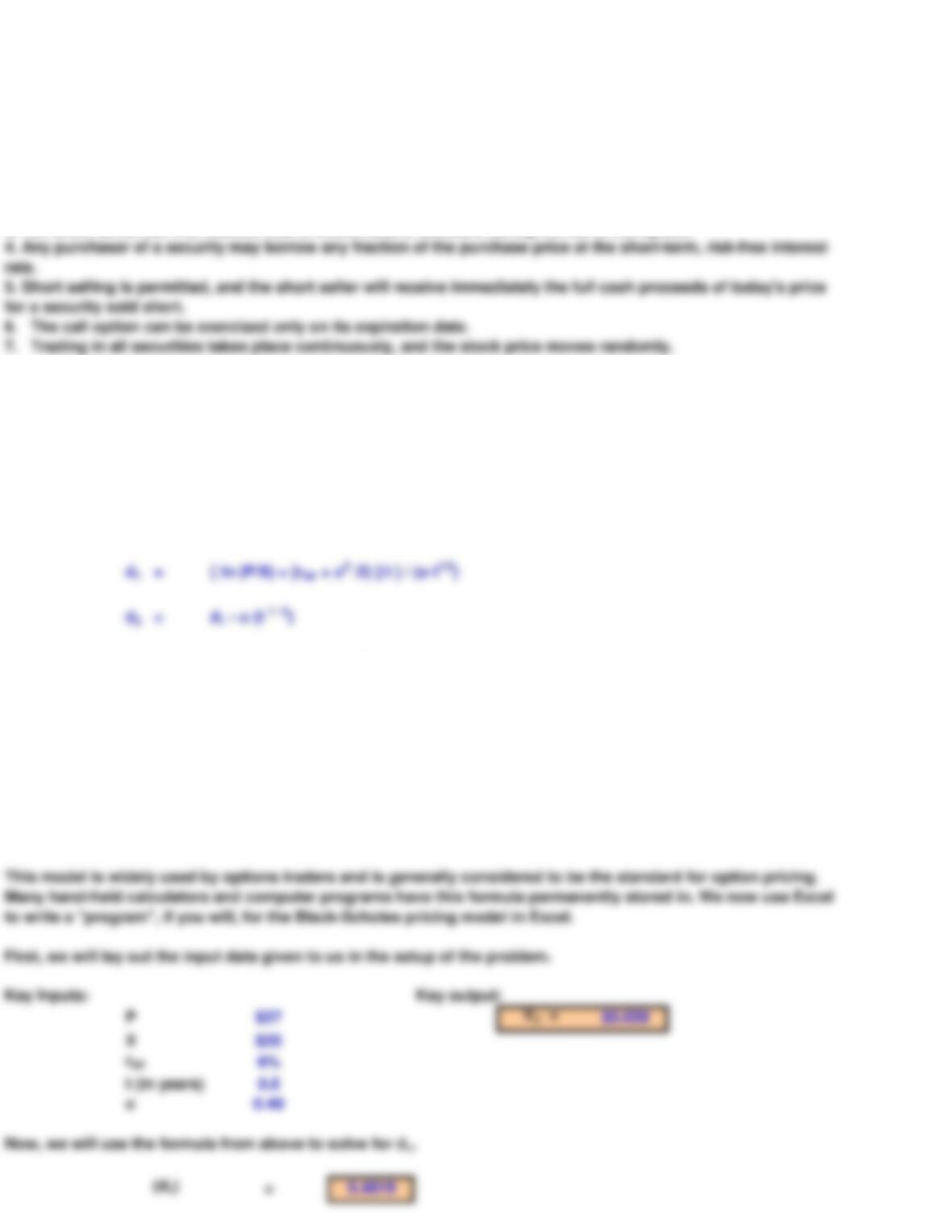
V =
P[ N (d1) ] – Xe-r t [ N (d2) ] Note: r is the risk-free rate.
to write a “program”, if you will, for the Black-Scholes pricing model in Excel.
First, we will lay out the input data given to us in the setup of the problem.
e. In 1973, Fischer Black and Myron Scholes developed the Black-Scholes Option Pricing Model (OPM).
In deriving this option pricing model, Black and Scholes made the following assumptions:
The derivation of the Black-Scholes model rests on the concept of a riskless hedge. By buying shares of a stock
and simultaneously selling call options on that stock, an investor can create a risk-free investment position,
where gains on the stock are exactly offset by losses on the option. Ultimately, the Black-Scholes model utilizes
these three formulas:
e. (1.) What assumptions underlie the OPM?
In these equations, V is the value of the option. P is the current price of the stock. N(d1) is the area beneath the
standard normal distribution corresponding to (d1). X is the strike price. rRF is the risk-free rate. t is the time to
maturity. N(d2) is the area beneath the standard normal distribution corresponding to (d2). s, or sigma, is the
volatility of the stock price, as measured by the standard deviation.
5. Short selling is permitted, and the short seller will receive immediately the full cash proceeds of today’s price
for a security sold short.
6. The call option can be exercised only on its expiration date.
7. Trading in all securities takes place continuously, and the stock price moves randomly.
4. Any purchaser of a security may borrow any fraction of the purchase price at the short-term, risk-free interest
e. (2.) Write out the three equations that constitute the model.
1. The stock underlying the call option provides no dividends or other distributions during the life of the option.
2. There are no transaction costs for buying or selling either the stock or the option.
3. The short-term, risk-free interest rate is known and is constant during the life of the option.
e. (3.) What is the value of the following call option according to the OPM?
Looking at these equations we see that you must first solve d1 and d2 before you can proceed to value the option.

Having solved for d1, we will now use this value to find d2.
(d2)=0.1355
At this point, we have all of the necessary inputs for solving for the value of the call option. We will use the
formula for V from above to find the value. The only complication arises when entering N(d1) and N(d2).
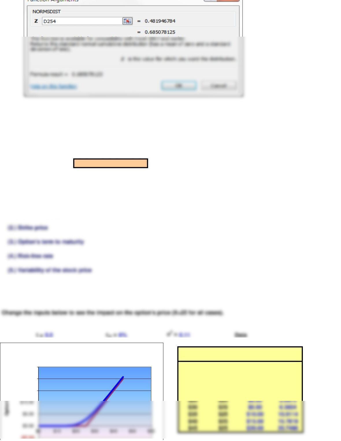
Using the NORMSDIST function:
(d1) = 0.6851
(d2) = 0.5539
VC = $5.06
(1.) Current stock price
Change the inputs below to see the impact on the option’s price (X=25 for all cases).
Price of Strike Exercise Option
the stock Price Value Price
$0 $25 $0.00 0.0000
$5 $25 $0.00 0.0000
$10 $25 $0.00 0.0001
$15 $25 $0.00 0.0330
$20 $25 $0.00 0.5932
$25 $25 $0.00 2.6873
$30 $25 $5.00 6.3654
Using the Black-Scholes formula and the cumulative distributions, we can solve for the option value.
EFFECTS OF OPM FACTORS ON THE VALUE OF A CALL OPTION
f. What impact does each of the following call option parameters have on the value of a call option? Answer:
See the sensitivity analysis below; also, see Chapter Mini Case Show
Let us now turn our attention to determining how sensitive the call option value is to the five factors of the Black-
Scholes OPM. We will set up data tables for each factor determining the call value if the specified input is
changed plus or minus 15% and 30%.
($5.00)
$15.00
$20.00
$25.00
Option Pricing: Sensitivity Analysis
(2.) Strike price
(3.) Option’s term to maturity
(4.) Risk-free rate
(5.) Variability of the stock price
g. What is put-call parity? Answer: See Chapter Mini Case Show
($5.00)
Stock Price
Exercise value Option price