CFIN6 – CHAPTER 8
INTEGRATIVE PROBLEM SOLUTION
a(1). The 8% T-bill return does not depend on the state of the economy because the Treasury must (and
will) redeem the bills at par regardless of the state of the economy.
The T-bills are risk-free in the default risk sense because the 8% return will be realized in all possible
a(2). High Tech’s returns move with, and thus are positively correlated with, the economy, because the firm’s
sales, and hence profits, generally will experience the same type of ups and downs as the economy. If the
economy is booming, so will High Tech. On the other hand, Collections is considered by many investors to
be a hedge against both bad times and high inflation; so if the stock market crashes, investors in this stock
should do relatively well. Stocks such as Collections are thus negatively correlated with (move counter to)
the economy. [Note: In actuality, it is almost impossible to find stocks that are expected to move counter to
the economy. Even Collections shares have positive (but low) correlation with the market.]
bills–T
r
ˆ
= 8.00%
sCollection
r
ˆ
= 1.74%
Rubber U.S.
r
ˆ
= 13.80%
M
r
ˆ
= 15.00%
c(1). The standard deviation is calculated as follows:
2 2 2 2 2
High Tech 2
0.1( 22.0% 17.4%) 0.2( 2.0% 17.4%) 0.4(20.0% 17.4%) 0.2(35.0% 17.4%)
0.1(50.0% 17.4%)
= − − + − − + − + −
+−
c(2). The standard deviation is a measure of a security’s (or a portfolio’s) total, or stand-alone, risk. The
larger the standard deviation, the higher the probability that actual realized returns will fall far below
the expected return, and that losses rather than profits will be incurred.
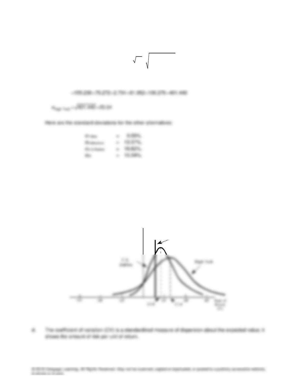
c(3). Probability distribution curves for High Tech, U.S. Rubber, and T–bills are shown here:
T-bills
Probability
n
22
ii
i1
ˆ
(r r)
=
= = −
Pr
Coefficient of CV
Variation ˆ
r
==
CVT-bills = 0.00%/8.00% = 0.00
CVHigh Tech = 20.04%/17.40% = 1.15
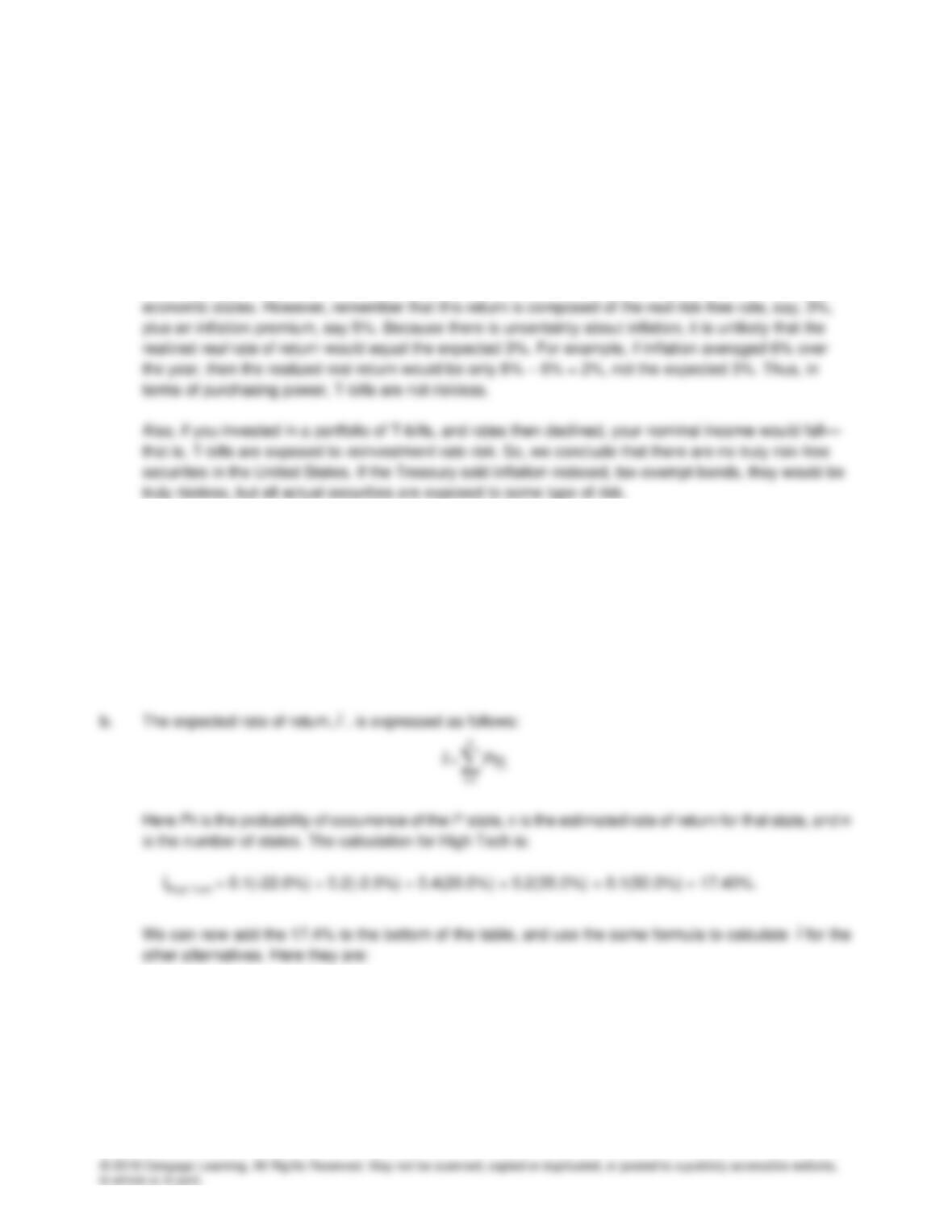
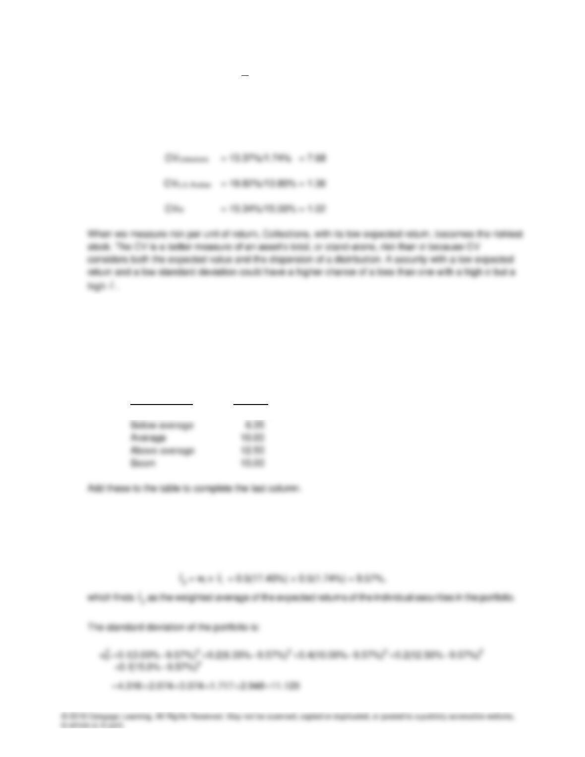
e(1). To find the expected rate of return on the two-stock portfolio, we first calculate the rate of return on the
portfolio in each state of the economy. Because we have half of our money in each stock, the
portfolio’s return will be a weighted average in each type of economy. For a recession, we have: rp =
0.5(-22%) + 0.5(28%) = 3%. We would do similar calculations for the other states of the economy, and
get these results:
State Portfolio
Recession 3.00%
Now multiply the probabilities times outcomes in each state to get the expected return on this two-stock
portfolio—that is, 3.0%(0.1) + 6.35%(0.2) + 10.0%(0.4) + 12.5%(0.2) + 15.0%(0.1) = 9.57%.
Alternatively, we could apply this formula:
P11.129 3.336% = =
CVP = 3.336%/9.57% = 0.349
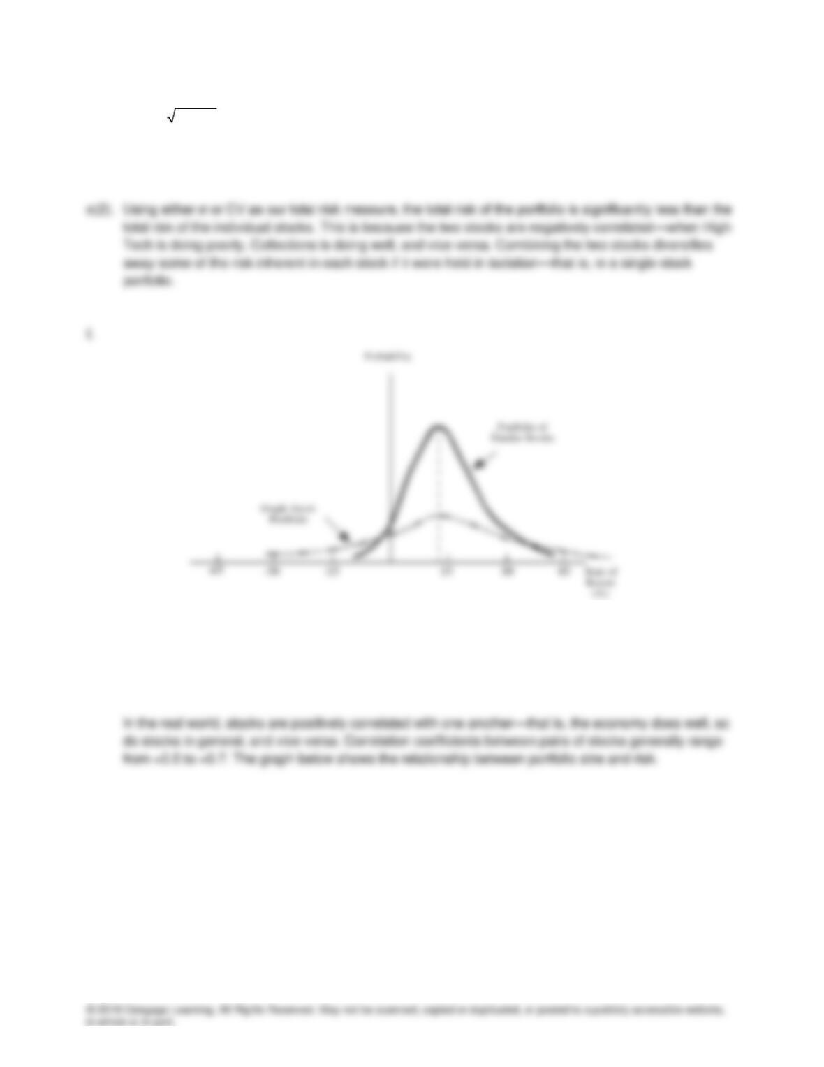
This graph shows the probability distributions for a one-stock portfolio and a portfolio of many similar
stocks. The graph shows that the standard deviation gets smaller as more stocks are combined in the
portfolio, while rp (the portfolio’s return) remains constant. Thus, by adding stocks to your portfolio,
which initially started as a single-stock portfolio, risk has been reduced.
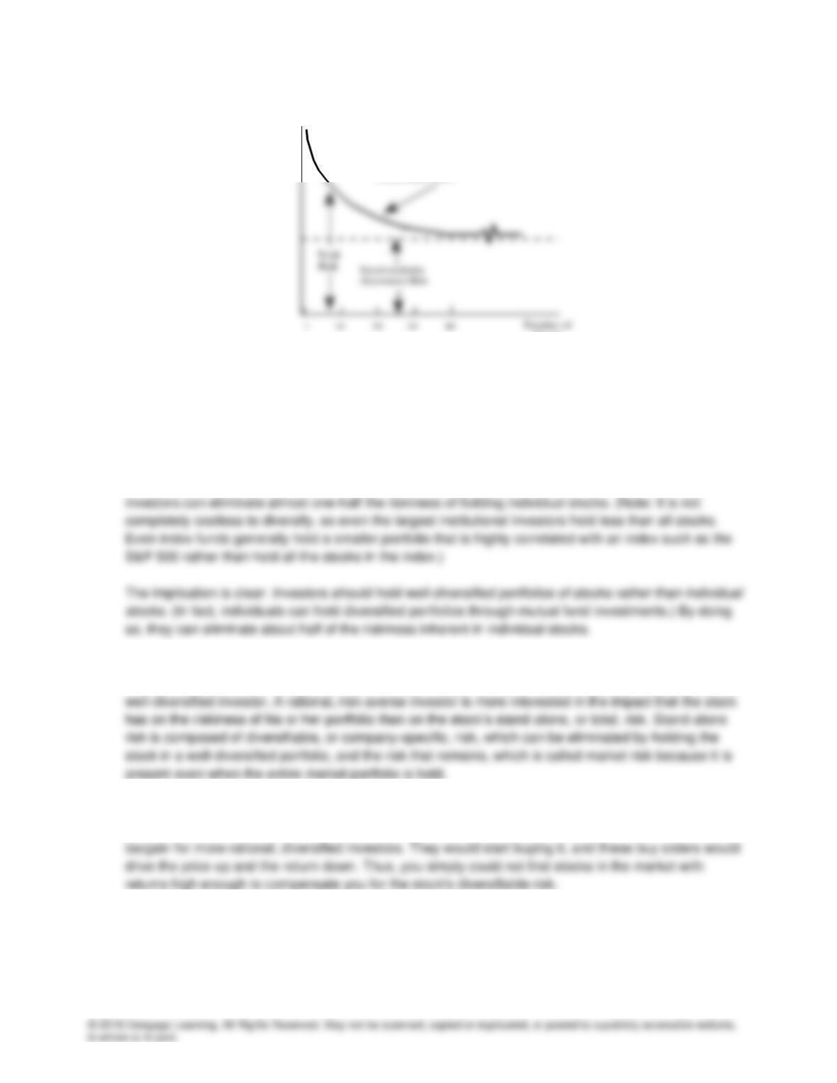
Portfolio
Risk, FP (%)
Stocks
Diversifiable
(Unsystematic) Risk
A single stock selected at random would on average have a standard deviation of approximately 30%.
As additional stocks are added to the portfolio, the portfolio’s standard deviation decreases because
the added stocks are not perfectly positively correlated. However, as more and more stocks are added,
each new stock has less of a risk-reducing impact, and eventually adding additional stocks has virtually
no effect on the portfolio’s risk as measured by σ. In fact, σ stabilizes at about 15% when 40 or more
randomly selected stocks are added. Thus, by combining stocks into well-diversified portfolios,
g(1). Portfolio diversification does affect investors’ views of risk. A stock’s total, or stand-alone, risk as
measured by its σ or CV, might be important to an undiversified investor, but it is not relevant to a
g(2). If you hold a one-stock portfolio, you will be exposed to a high degree of risk, but you won’t be
compensated for it. If the return were high enough to compensate you for your high risk, it would be a
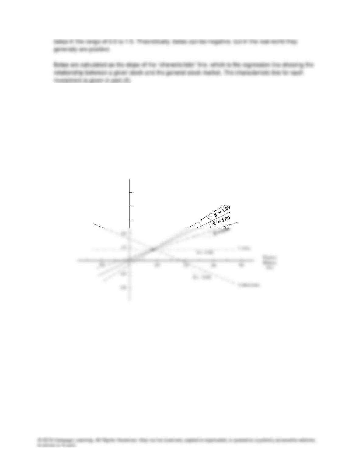
h(1). Draw the framework of the graph, put up the data, plot the points for the market (45° line) and connect
them, and then get the slope as δY/δX = 1.0. State that an average stock, by definition, moves with the
market. Then do the same with High Tech and U.S. Rubber. Beta coefficients measure the relative
volatility of a given stock vis-a-vis an average stock. The average stock’s beta is 1.0. Most stocks have
h(2). The expected returns are related to each alternative’s market risk—that is, the higher the alternative’s
rate of return the higher its beta. Also, note that T-bills have 0 risk.
h(3). We do not yet have enough information to choose among the various alternatives. We need to know
the required rates of return on these alternatives and compare them with their expected returns.
h(4).
50
40
30
Stock
Return
(%)
High Tech
Market
U.S. Rubber
Characteristic Lines
i(1). Here is the SML equation:
rj = rRF + (rM – rRF)βj.
If we use the T-bill yield as a proxy the risk-free rate, then rRF = 8%. Further, our estimate of rM =
r
ˆ
is
15%. Thus, the SML is drawn as follows:
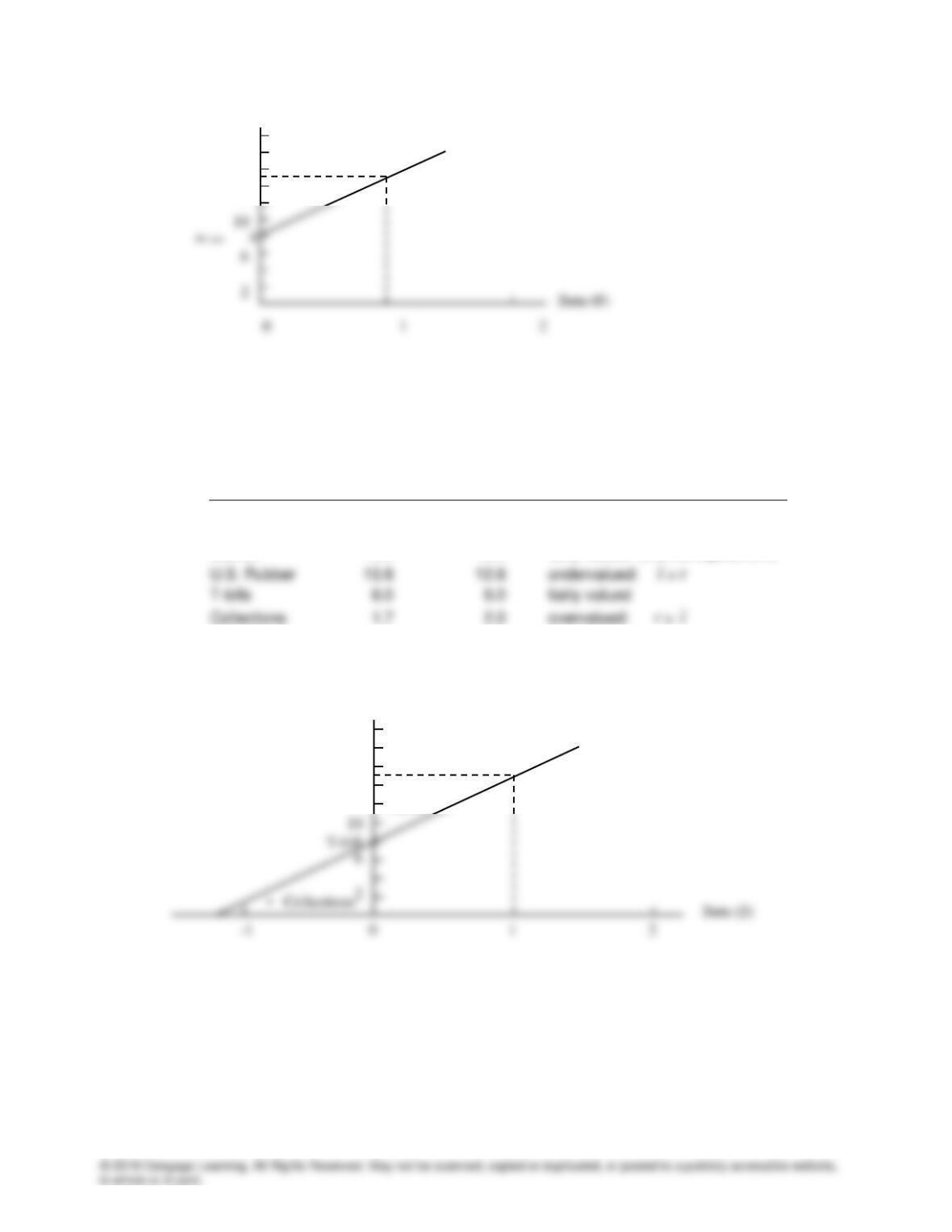
rT-bill = 8
i(2). Using the SML equation, we have the following relationships:
Expected Required
Return Return
Security (
r
ˆ
) (r) Condition
High Tech 17.4% 17.0% undervalued:
r
ˆ
r
ˆ
r
ˆ
> r
Market 15.0 15.0 fairly valued (market equilibrium)
T-bill •
These returns are plotted on the SML graph next.
The T-bills and market portfolio plot on the SML, High Tech and U.S. Rubber plot above it, and
Collections plots below it. Thus, the T-bills and the market portfolio promise a fair return, High Tech
and U.S. Rubber are good deals because they have expected returns above their required returns, and
Collections has an expected return below its required return.
i(3). Collections is an interesting stock. Its negative beta indicates negative market risk—including it in a
r (%)
18
14
SML
rM = 15
r (%)
18
14
SML
High Tech •
U.S.
Rubber •
Market •
portfolio of “normal” stocks will lower the portfolio’s risk. Therefore, its required rate of return is below
the risk-free rate. Basically, this means that Collections is a valuable security to rational,
well-diversified investors. To see why, consider this question: Would any rational investor ever make
an investment that has a negative expected return? The answer is “yes”—just think of the purchase of
i(4). Note that the beta of a portfolio is simply the weighted average of the betas of the stocks in the
portfolio. Thus, the beta of a portfolio with 50% High Tech and 50% Collections is:
βp = 0.5(βHigh Tech) + 0.5(βCollections) = 0.5(1.29) + 0.5(–0.86) = 0.215,
and the portfolio’s required return is 9.51%:
For a portfolio consisting of 50% High Tech plus 50% U.S. Rubber, the required return would be
14.90%:
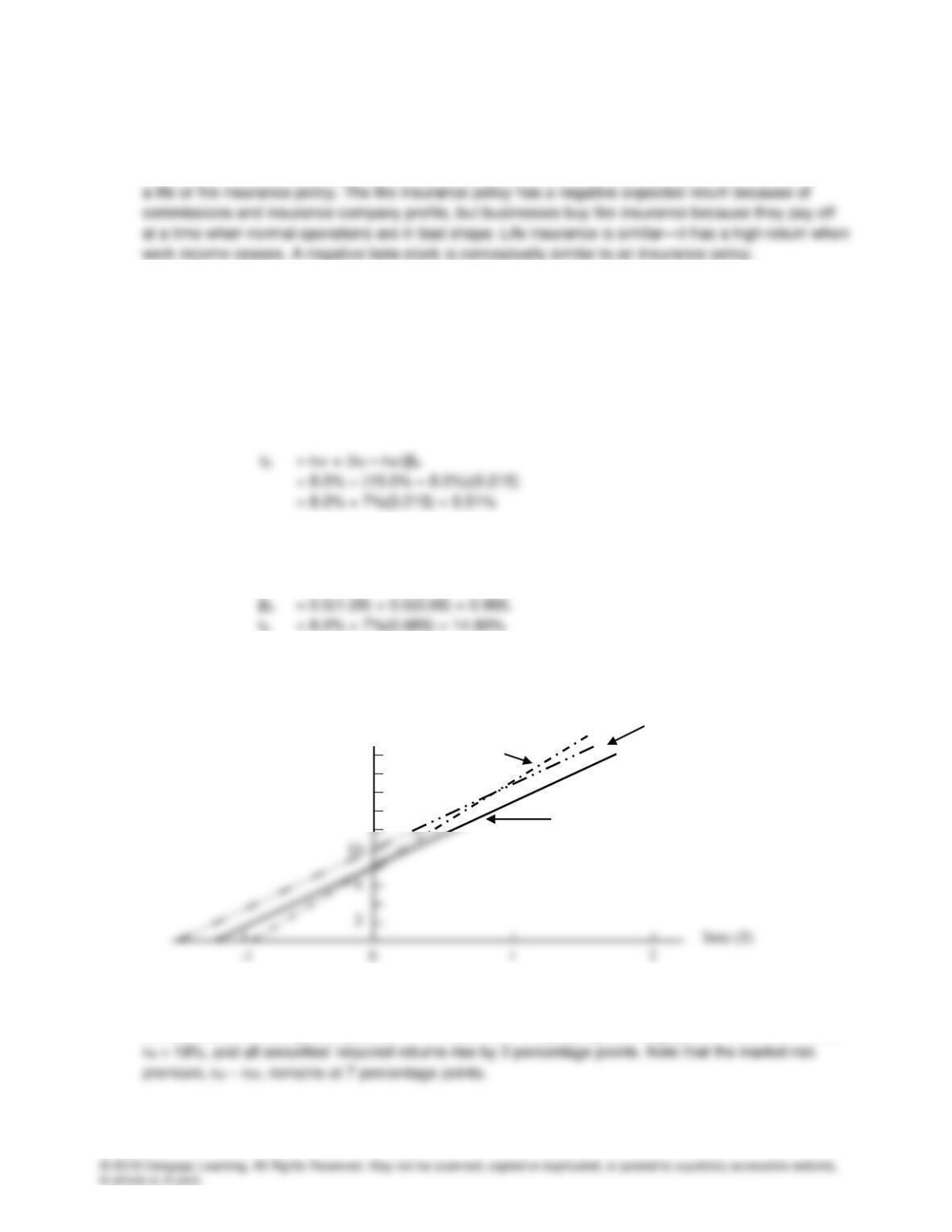
j(1). This effect is graphed next.
Here we have plotted the SML for betas ranging from 0 to 2.0. The base case SML is based on rRF =
8% and rM = 15%. If inflation expectations increase by 3%, with no change in risk aversion, then the
entire SML is shifted upward (parallel to the base case SML) by 3 percentage points. Now, rRF = 11%,
-1 0 1 2
r (%)
18
14
Original Situation
Increased Inflation
Increased Risk
Aversion

j(2). When investors’ risk aversion increases, the SML is rotated upward about the Y-intercept (rRF). rRF