7 – 12
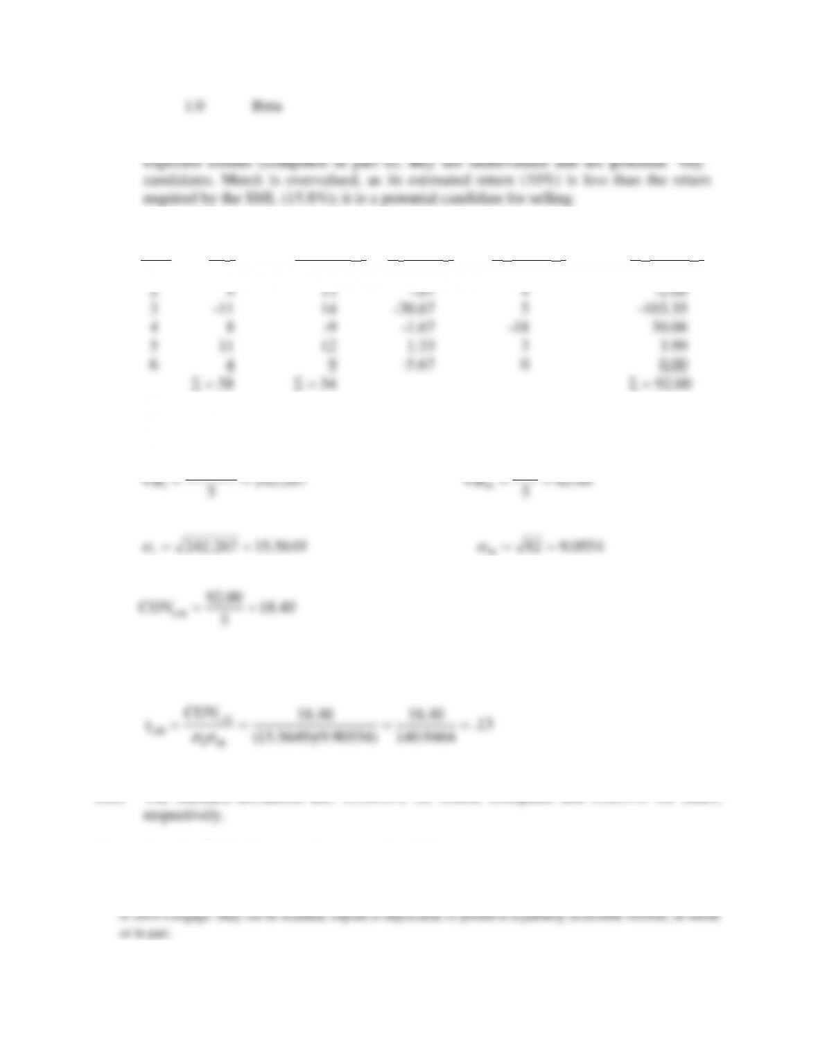
Intel, Ford, and Anheuser all have estimated return (given in part c) exceeding their
5. Chelle General (R1 – E(R1) x
Year (R1) Index (RM) R1 – E(R1) RM – E(RM) RM – E(RM)
1 37 15 27.33 6 163.98
E(R1) = 9.67 E(M) = 9
5(a). The correlation coefficient can be computed as follows:
5(b). The standard deviations are: 15.5649% for Chelle Computer and 9.0554% for index,
5(c). Beta for Chelle Computer is computed as follows:
00.82
5
410
Var 267.242
5
33.1211
Var M1 ====
40.18
5
00.92
COV M1, ==
13.
9464.140
40.18
)90554.9)(5649.15(
40.18
COV
r
M1
M1,
M1, ====
6.
6(a). Security Market Line
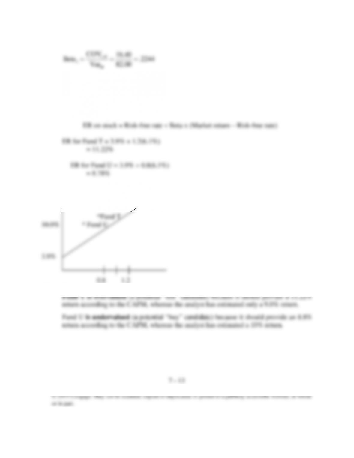
i. Fair-value plot. The following template shows, using the CAPM, the expected
return, ER, of Fund T and Fund U on the SML. The points are consistent with the
following equations:
ii. Analyst estimate plot. Using the analyst’s estimates, Fund T plots below the SML
and Fund U, above the SML.
6(b). Over vs. Undervalue
2244.
00.82
40.18
Var
COV
Beta
M
M1,
1===

7 – 14
7. R
1.0 Beta
7(b). = Cov i,m/(m)2
From a spreadsheet program, we find for Radar Tire and the Proxy,
7(c). Using the proxy:
E(RR) = 0.08 + 0.984(0.12 – 0.08)
8.
8(a). In general, for the APT, E(Rq) = 0 + 1bq1 + 2bq2
For security J:
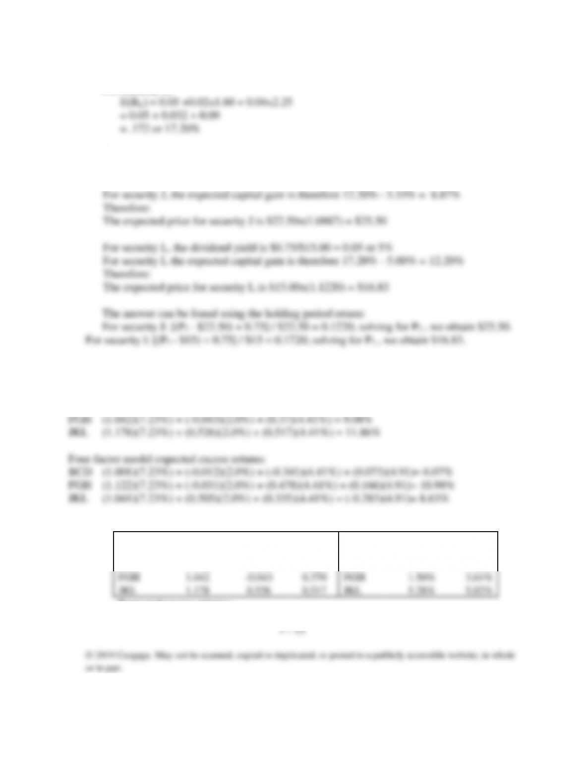
For Security L:
8(b). Total return = dividend yield + capital gain yield
For security J, the dividend yield is $0.75/$22.50 = 0.033 or 3.33%
9.
9 (a).
Three-factor model expected excess returns:
BCD (0.966)(7.23%) + (-0.018)(2.0%) + (-0.388)(4.41%) = 5.24%
9(b).
Coefficients
Factor Risk Premia
3 -factor
MKT
SMB
HML
30-year
80-year
BCD
0.966
-0.018
-0.388
BCD
7.11%
7.92%
FGH
1.042
-0.043
0.370
FGH
1.50%
3.61%
JKL
1.178
0.526
0.517
JKL
5.28%
5.02%
Expected excess returns:

Using factor premium from:
30-year
80-year
BCD
4.79%
5.64%
CSX
9.30%
9.95%
JKL
11.89%
13.82%
Sample calculation:
BCD, using 30-year premia:
9(c).
coefficients
Factor Risk Premia
4-factor
MKT
SMB
HML
MOM
30-year
80-year
BCD
0.777
-0.655
-0.186
-0.074
BCD
7.11%
7.92%
FGH
0.593
-0.123
0.084
0.042
FGH
1.50%
3.61%
JKL
0.804
0.100
0.496
-0.158
JKL
5.28%
5.02%
Expected excess returns:
Using factor premium from:
30-year
80-year
BCD
2.97%
2.13%
FGH
4.81%
5.09%
JKL
7.22%
7.67%
9(d). The excess returns for all the stocks for both periods seem moderately large. This is partly
10(a). RQRS = 4.5 +7.5×1.24
RTUV = 4.5 + 7.5×0.91
= 4.5 + 6.825

7 – 17
10(b). RQRS = 4.5 + 7.5×1.24 + (-0.3)x(-0.42) + 0.6×0.00
RTUV = 4.5 + 7.5×0.91 + (-0.3)x(0.54) + 0.6×0.23
= 12.252%
10(c). Assuming that the factor loadings are significant, the three-factor model should be more
10(d). Because the factor loadings on MACRO2 are zero for two of the stocks, it appears that
11(a). E(RD) = 5.0 + 1.21 + 3.42 = 13.1%
E(RE) = 5.0 + 2. + 2. =
Solving the second equation for 1 in terms of 2, we get:
11(b). Because neither stock pays a dividend, the total return is all due to price appreciation.
Therefore for stock D:

11(c). From part (a), the risk premium for factor 1 was 2.5%. The new risk factor is thus 2.5% +
0.25%, or 2.75%. The new expected returns are:
E(RD) = 5.0 + (1.2×2.75) +(3.4×1.5)
11(d). D: PD0(1 + 0.134) = $55
PD0 = $55/1.134
12(a). Because no stock pays a dividend, all return is due to price appreciation.
E(RA) = 1.1×0.04 + 0.8×0.02
= 0.044 + 0.016
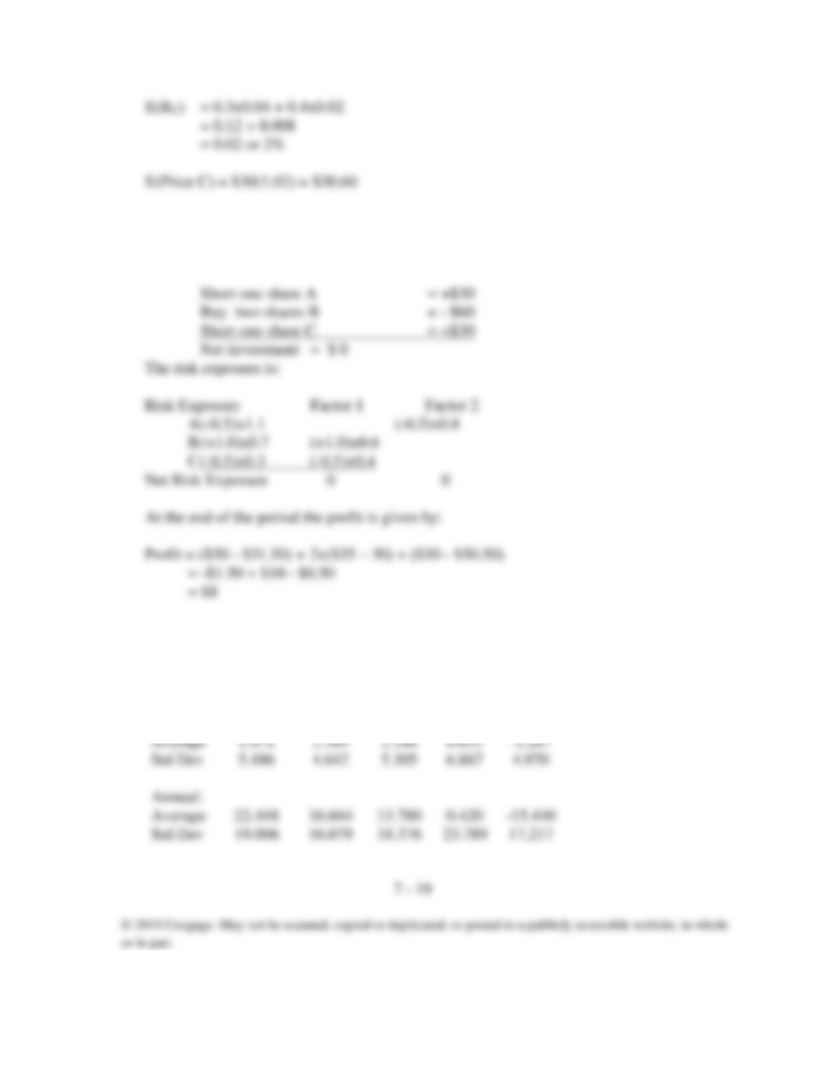
12(b). In order to create a riskless arbitrage investment, an investor would short one share of A
and one share of C and buy two shares of B. The weights of this portfolio are WA = -0.5,
WB = +1.0, and WC = -0.5. The net investment is:
13.
13(a). Using a spreadsheet program, we compute the following:
Portfolio
A
Portfolio
B
Factor
1
Factor
2
Factor
3
Monthly:
Average
1.871
1.389
1.148
0.035
-1.287
Std Dev
5.486
4.642
5.305
6.867
4.970
Annual:
Average
22.448
16.664
13.780
0.420
-15.440
Std Dev
19.006
16.079
18.376
23.789
17.217
7 – 20
13(b). No, it is not clear. Portfolio A earned a higher return than Portfolio B but also had higher
13(c). Using a spreadsheet program, we obtain:
correlation between 1&2: 0.2207
13(d). In theory the correlations should be zero because we want the factors to be independent
of each other.
13(e). Factors 1 and 2 are not highly correlated, but it appears that there is significant correlation
between factors 1 and 3 and factors 2 and 3. Statistically speaking, this leads to problems
of multicollinearity, which would affect regression estimates.
14.
14(a). Using a basic regression package, we get the following results (t-statistics given in
parentheses):
14(b). The adjusted R2’s in both regressions are very high (.967 and .905, respectively.) This
14(c). Factor 1 is the most likely candidate for the market factor because it has a large,
significant, and positive effect on both portfolios. Factors 2 and 3 have different signs in
the two equations.

7 – 21