CHAPTER 7
RISK ANALYSIS, REAL OPTIONS, AND
CAPITAL BUDGETING
Answers to Concepts Review and Critical Thinking Questions
2. With a sensitivity analysis, one variable is examined over a broad range of values. With a scenario
analysis, all variables are examined for a limited range of values.
3. It is true that if average revenue is less than average cost, the firm is losing money. This much of the
4. From the shareholder perspective, the financial break-even point is the most important. A project can
5. The project will reach the cash break-even first, the accounting break-even next, and finally the
financial break-even. For a project with an initial investment and sales afterwards, this ordering will
6. Traditional NPV analysis is often too conservative because it ignores profitable options such as the
7. The type of option most likely to affect the decision is the option to expand. If the country just
9. There are two sources of value with this decision to wait. The price of the timber can potentially
10. Option analysis should stop when the additional analysis has a negative NPV. Since the additional
analysis is likely to occur almost immediately, then it would have a negative NPV when the benefits
Solutions to Questions and Problems
NOTE: All end-of-chapter problems were solved using a spreadsheet. Many problems require multiple
steps. Due to space and readability constraints, when these intermediate steps are included in this solutions
manual, rounding may appear to have occurred. However, the final answer for each problem is found
without rounding during any step in the problem.
Basic
1. a. To calculate the accounting break-even, we first need to find the depreciation for each year. The
depreciation is:
Depreciation = $604,000/8
Depreciation = $75,500 per year
b. We will use the tax shield approach to calculate the OCF. The OCF is:
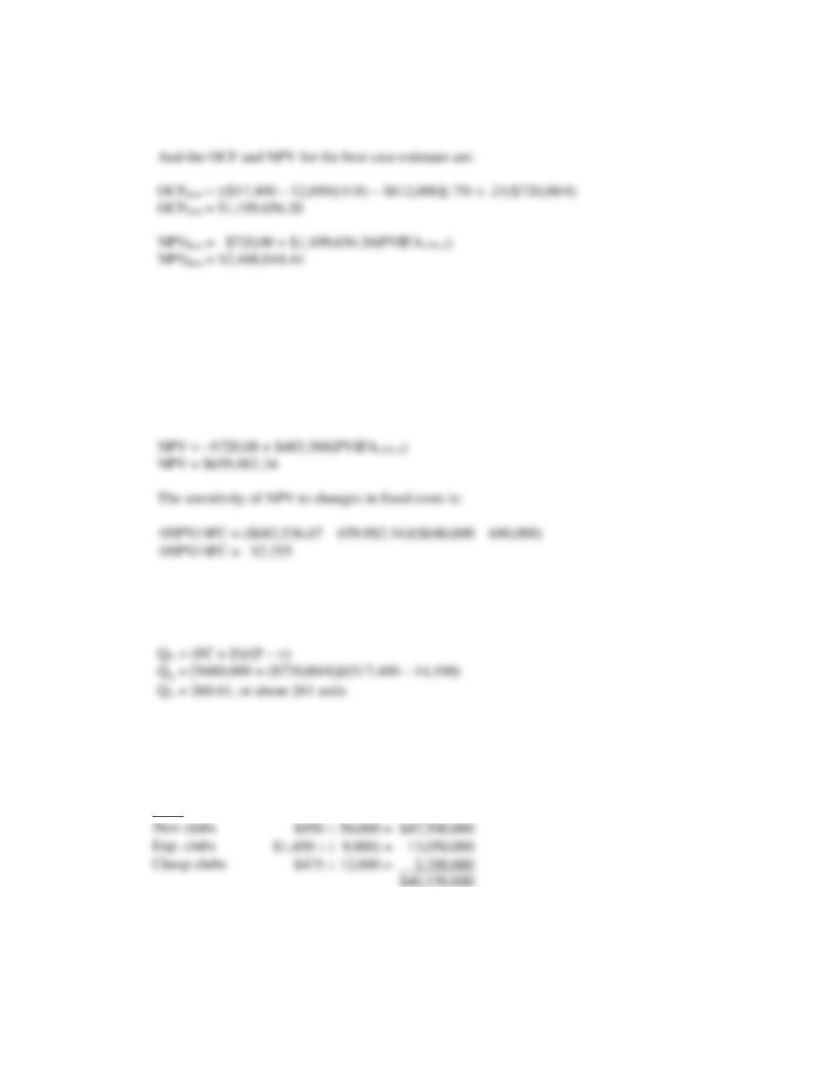
OCFbase = [(P – v)Q – FC](1 – TC) + TCD
OCFbase = [($36 – 17)(55,000) – $685,000](.79) + .21($75,500)
OCFbase = $300,255
To calculate the sensitivity of the NPV to changes in the quantity sold, we will calculate the NPV
at a different quantity. We will use sales of 56,000 units. The OCF at this sales level is:
And the NPV is:
So, the change in NPV for every unit change in sales is:
c. To find out how sensitive OCF is to a change in variable costs, we will compute the OCF at a
variable cost of $18. Again, the number we choose to use here is irrelevant: We will get the same
ratio of OCF to a one dollar change in variable cost no matter what variable cost we use. So,
using the tax shield approach, the OCF at a variable cost of $18 is:
OCFnew = [($36 – 18)(55,000) – 685,000](.79) + .21($75,500)
OCFnew = $256,805
2. We will use the tax shield approach to calculate the OCF for the best– and worst-case scenarios. For
the best-case scenario, the price and quantity increase by 10 percent, so we will multiply the base case
numbers by 1.1, a 10 percent increase. The variable and fixed costs both decrease by 10 percent, so
we will multiply the base case numbers by .9, a 10 percent decrease. Doing so, we get:
3. We can use the accounting break-even equation:
QA = (FC + D)/(P – v)
to solve for the unknown variable in each case. Doing so, we find:
4. When calculating the financial break-even point, we express the initial investment as an equivalent
annual cost (EAC). Dividing the initial investment by the 5-year annuity factor, discounted at 12
percent, the EAC of the initial investment is:
EAC = Initial Investment/PVIFA12%,5
EAC = $435,000/3.60478
5. If we purchase the machine today, the NPV is the cost plus the present value of the increased cash
flows, so:
NPV0 = –$2,800,000 + $435,000(PVIFA9%,10)

We should not necessarily purchase the machine today. We would want to purchase the machine when
the NPV is the highest. So, we need to calculate the NPV each year. The NPV each year will be the
cost plus the present value of the increased cash savings. We must be careful, however. In order to
make the correct decision, the NPV for each year must be taken to a common date. We will discount
all of the NPVs to today. Doing so, we get:
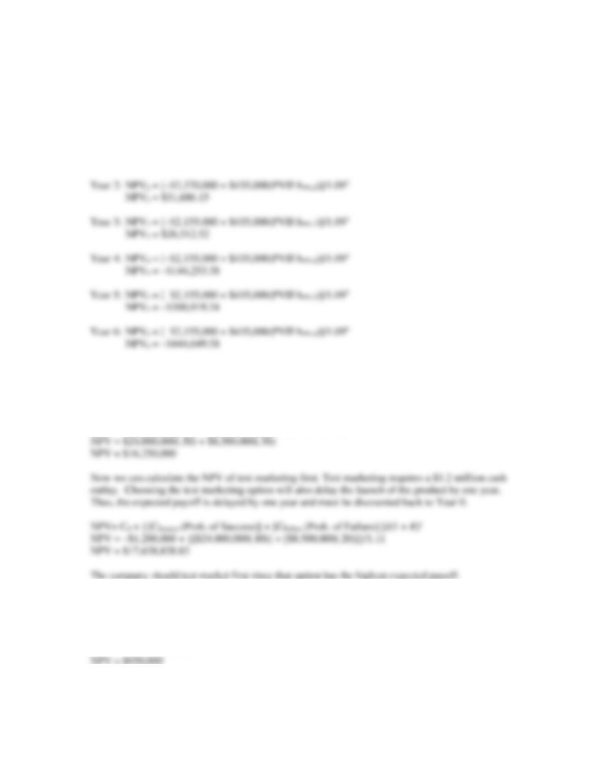
Year 1: NPV1 = [–$2,585,000 + $435,000(PVIFA9%,9)]/1.09
NPV1 = $21,038.90
The company should purchase the machine in Year 2 when the NPV is the highest.
6. We need to calculate the NPV of the two options: Go directly to market now, or utilize test
marketing first. The NPV of going directly to market now is:
NPV = CSuccess (Prob. of Success) + CFailure (Prob. of Failure)
7. We need to calculate the NPV of each option, and choose the option with the highest NPV. So, the
NPV of going directly to market is:
NPV = CSuccess (Prob. of Success)
NPV = $1,900,000(.50)
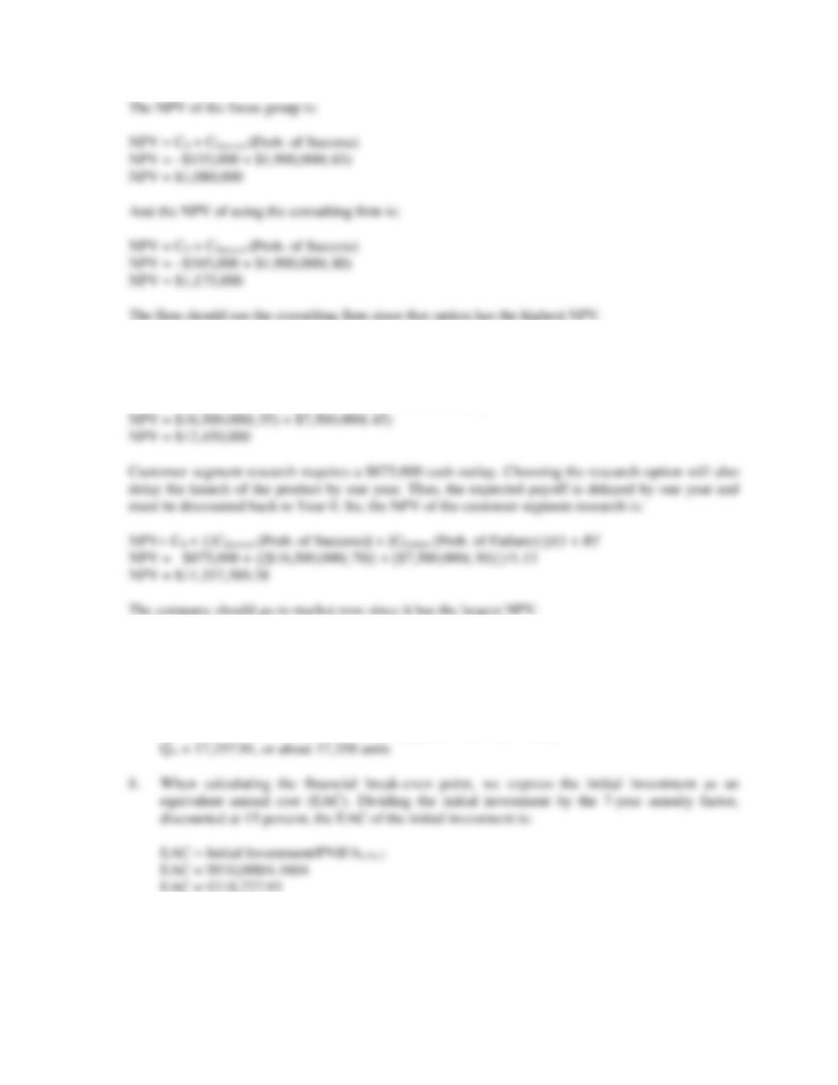
8. The company should analyze both options, and choose the option with the greatest NPV. So, if the
company goes to market immediately, the NPV is:
NPV = CSuccess (Prob. of Success) + CFailure (Prob. of Failure)
9. a. The accounting break-even is the aftertax sum of the fixed costs and depreciation charge divided
by the aftertax contribution margin (selling price minus variable cost). So, the accounting break–
even level of sales is:
QA = [(FC + Depreciation)(1 – TC)]/[(P – VC)(1 – TC)]
QA = [($435,000 + $910,000/7) (1 – .21)]/[($43 – 10.45)(1 – .21)]
10. When calculating the financial break-even point, we express the initial investment as an equivalent
annual cost (EAC). Dividing the initial investment by the 5-year annuity factor, discounted at 8
percent, the EAC of the initial investment is:
EAC = Initial Investment/PVIFA8%,5
EAC = $530,000/3.99271
EAC = $132,741.92
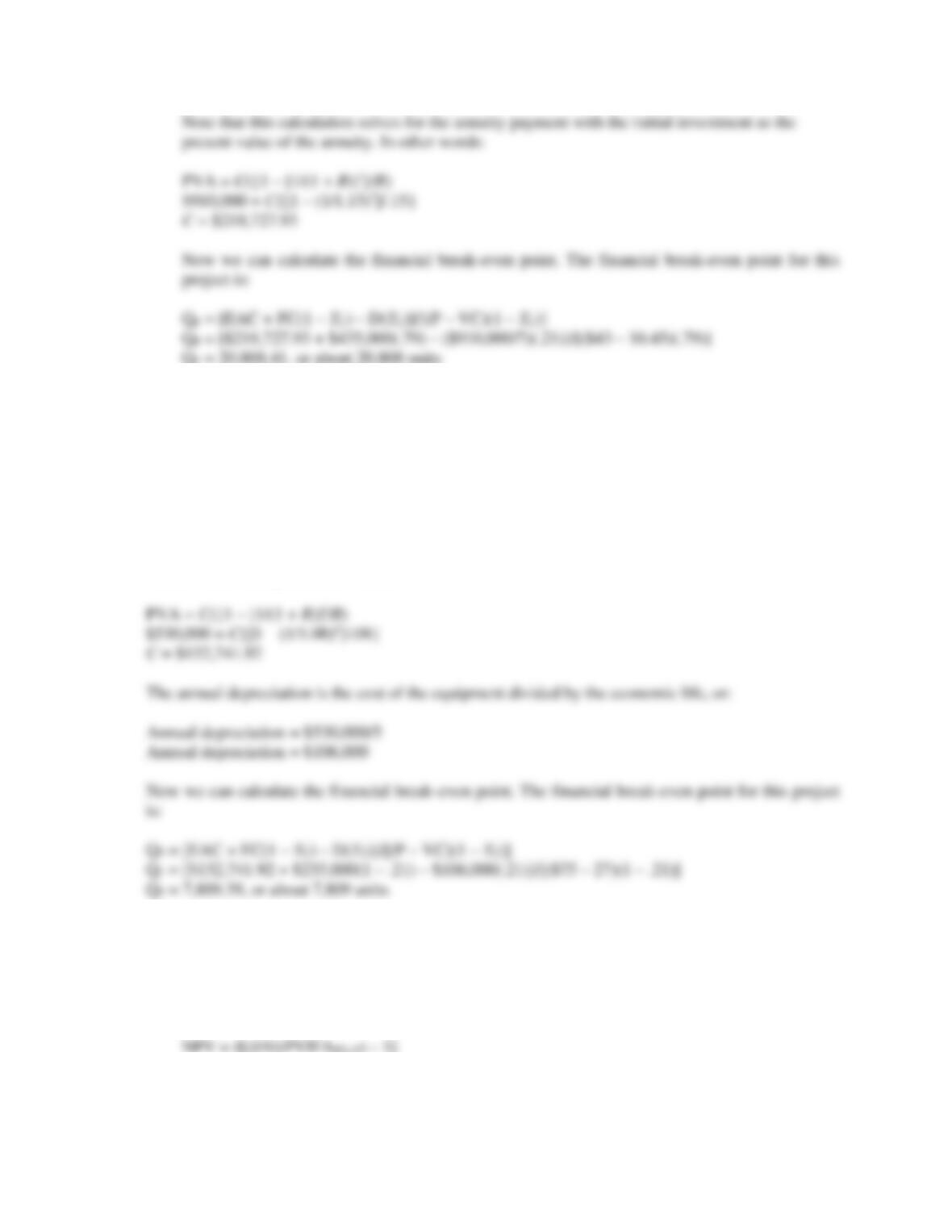
Note that this calculation solves for the annuity payment with the initial investment as the present
value of the annuity. In other words:
Intermediate
11. a. At the accounting break-even, the IRR is zero percent since the project recovers the initial
investment. The payback period is N years, the length of the project since the initial investment
is exactly recovered over the project life. The NPV at the accounting break-even is:
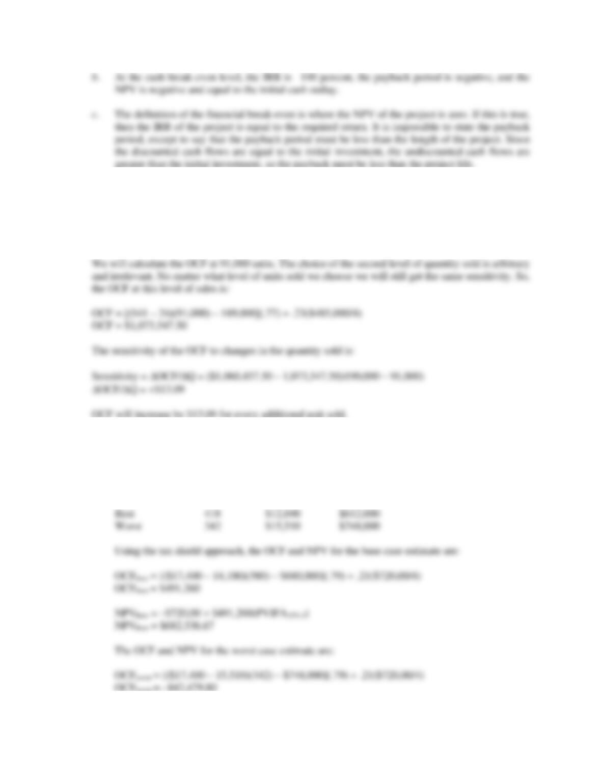
12. Using the tax shield approach, the OCF at 90,000 units will be:
OCF = [(P – v)Q – FC](1 – TC) + TC(D)
OCF = [($41 – 24)(90,000) – 189,000](.77) + .23($485,000/4)
OCF = $1,060,457.50
13. a. The base-case, best-case, and worst-case values are shown below. Remember that in the best-
case, unit sales increase, while costs decrease. In the worst-case, unit sales decrease and costs
increase.
Scenario Unit sales Variable cost Fixed costs
Base 380 $14,100 $680,000
NPVworst = –$720,00 – $42,479.80(PVIFA15%,4)
NPVworst = –$841,278.91
b. To calculate the sensitivity of the NPV to changes in fixed costs, we choose another level of fixed
costs. We will use fixed costs of $690,000. The OCF using this level of fixed costs and the other
base case values with the tax shield approach is:
OCF = [($17,400 – 14,100)(380) – $690,000](.79) + .21($720,00/4)
OCF = $483,360
And the NPV is:
For every dollar FC increase, NPV falls by $2.255.
c. The accounting break-even is:
14. The marketing study and the research and development are both sunk costs and should be ignored. We
will calculate the sales and variable costs first. Since we will lose sales of the expensive clubs and gain
sales of the cheap clubs, these must be accounted for as erosion. The total sales for the new project
will be:
Sales
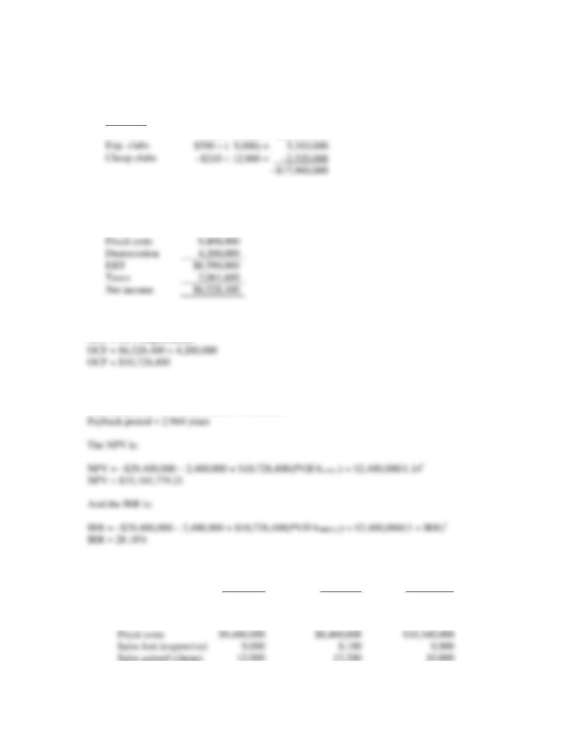
For the variable costs, we must include the units gained or lost from the existing clubs. Note that the
variable costs of the expensive clubs are an inflow. If we are not producing the sets any more, we will
save these variable costs, which is an inflow. So:
Var. costs
New clubs
–$415 50,000 = –$20,750,000
The pro forma income statement will be:
Sales
$40,150,000
Variable costs
17,960,000
Depreciation
Taxes
Using the bottom up OCF calculation, we get:
So, the payback period is:
Payback period = 2 + $10,343,200/$10,728,400
15. The upper and lower bounds for the variables are:
Base Case Best Case Worst Case
Unit sales (new) 50,000 55,000 45,000
Price (new) $950 $1,045 $855
VC (new) $415 $374 $457
Cheap clubs
–$210 12,000 = –2,520,000
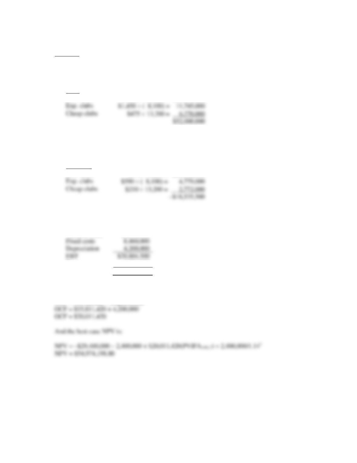
Best-case
We will calculate the sales and variable costs first. Since we will lose sales of the expensive clubs and
gain sales of the cheap clubs, these must be accounted for as erosion. The total sales for the new project
will be:
Sales
New clubs
$1,045 55,000 = $57,475,000
For the variable costs, we must include the units gained or lost from the existing clubs. Note that the
variable costs of the expensive clubs are an inflow. If we are not producing the sets any more, we will
save these variable costs, which is an inflow. So:
Var. costs
New clubs
–$374 55,00 = –$25,542,500
Exp. clubs
The pro forma income statement will be:
Sales
$52,000,000
Variable costs
18,535,500
Depreciation
4,200,000
EBT
$20,804,500
Taxes
4,993,080
Net income
$15,811,420
Using the bottom up OCF calculation, we get:
OCF = Net income + Depreciation
Exp. clubs
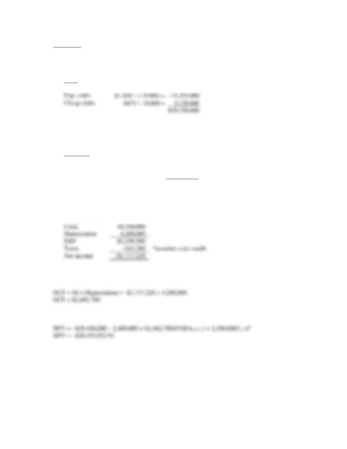
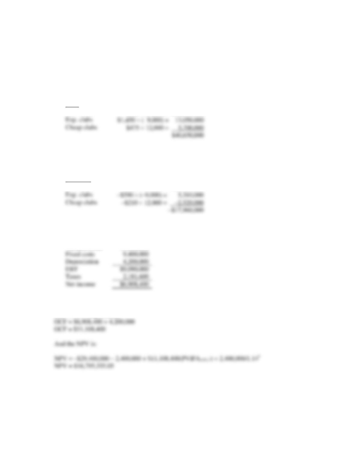
Worst-case
We will calculate the sales and variable costs first. Since we will lose sales of the expensive clubs and
gain sales of the cheap clubs, these must be accounted for as erosion. The total sales for the new project
will be:
Sales
New clubs
$855 45,000 = $38,475,000
For the variable costs, we must include the units gained or lost from the existing clubs. Note that the
variable costs of the expensive clubs are an inflow. If we are not producing the sets any more, we will
save these variable costs, which is an inflow. So:
Var. costs
New clubs
–$457 45,000 = –$20,542,500
Exp. clubs
–$590 (–9,900) = 5,841,000
Cheap clubs
–$210 10,800 = –2,268,000
–$16,969,500
The pro forma income statement will be:
Sales
$29,250,000
Variable costs
16,969,500
Costs
EBT
Taxes
*assumes a tax credit
Net income
Using the bottom up OCF calculation, we get:
And the worst-case NPV is:
Exp. clubs
Cheap clubs
16. To calculate the sensitivity of the NPV to changes in the price of the new club, we need to change the
price of the new club. We will choose $960, but the choice is irrelevant as the sensitivity will be the
same no matter what price we choose.
We will calculate the sales and variable costs first. Since we will lose sales of the expensive clubs and
gain sales of the cheap clubs, these must be accounted for as erosion. The total sales for the new project
will be:
Sales
New clubs
$960 50,000 = $48,000,000
For the variable costs, we must include the units gained or lost from the existing clubs. Note that the
variable costs of the expensive clubs are an inflow. If we are not producing the sets any more, we will
save these variable costs, which is an inflow. So:
Var. costs
New clubs
–$415 50,000 = –$20,750,000
Exp. clubs
Cheap clubs
The pro forma income statement will be:
Sales
$40,650,000
Variable costs
17,960,000
Fixed costs
Depreciation
EBT
Taxes
Net income
Using the bottom up OCF calculation, we get:
OCF = NI + Depreciation
Exp. clubs
Cheap clubs