A6-12. Ignoring Intel, Exxon seems to be the most attractive stock because of the remaining 9
Q6-13. Classify each of the following events as a source of systematic or unsystematic risk.
a. Ben Bernanke retires as Chairman of the Federal Reserve and Arnold Schwarzenegger
A6-13. a, c, and e are systematic risks because they affect most firms in the market. Item b pri-
marily affects Martha Stewart’s company, and likewise, d mainly affects the firm involved
Answers to End-of-Chapter Problems
Understanding Returns
P6-1. You purchase 1,000 shares of Spears Grinders Inc. stock for $45 per share. A year later, the
stock pays a dividend of $1.25 per share and it sells for $49.
a. Calculate your total dollar return.
b. Calculate your total percentage return.
c. Do the answers to parts (a) and (b) depend on whether you sell the stock after one year
or continue to hold it?
P6-2. A financial adviser claims that a particular stock earned a total return of 10 % last year.
During the year the stock price rose from $30 to $32.50. What dividend did the stock pay?
P6-3. D. S. Trucking Company stock pays a $1.50 dividend every year. A year ago the stock sold
for $25 per share, and its total return during the past year was 20%. What does the stock
sell for today?
P6-4. Nano-Motors Corp. has stock outstanding which sells for $10 per share. Macro-Motors Inc.
shares cost $50 each. Neither stock pays dividends at present.
a. An investor buys 100 shares of Nano-Motors. A year later the stock sells for $15. Cal-
culate the total return in dollar terms and in percentage terms.
Chapter 6 The Trade-Off Between Risk and Return 167
b. Another investor buys 100 shares of Macro-Motors stock. A year later the stock has
risen to $56. Calculate the total return in dollar terms and in percentage terms.
c. Why is it difficult to say which investor had a better year?
A6-4. a. Total dollar return = $500. Total % return = 50%.
P6-5. David Rawlings pays $1,000 to buy a five-year Treasury bond that pays a 6% coupon rate
(for simplicity, assume annual coupon payments). One year later, the market’s required re-
turn on this bond has increased from 6% to 7%. What is Rawlings’ total return (in dollar
and percentage terms) on the bond?
P6-6. G. Welch purchases a corporate bond that was originally issued for $1,000 several years
ago. The bond has four years remaining until it matures, the market price now is $1,054.45,
and the yield-to–maturity (YTM) is 4%. The bond pays an annual coupon of $55 with the
next payment due in one year.
a. What is the bond’s coupon rate? Its coupon yield?
b. Suppose Welch holds this bond for one year and the YTM does not change. What is
the total percentage return on the bond? Show that on a percentage basis, the total re-
turn is the sum of the interest and capital gain/loss components.
c. If the yield-to-maturity decreases during the first year from 4% to 3.5 %, what is the
total percentage return that year?
b. At the end of one year if the YTM is still four percent, the price will be $1,041.63. The
total percentage return will be ($1,041.63 + $55 − $1,054.45)/$1,054.45 = 4%. That
should not be a surprise. The bond provides a return that exactly equals the return re-
168 Instructor’s Manual
P6-7. In this advanced problem, let’s look at the behavior of ordinary Treasury bonds and infla-
tion-indexed bonds, or TIPS. We will simplify by assuming annual interest payments ra-
ther than semiannual. Suppose over the next five years, investors expect 3 % inflation each
year. The Treasury issues a five-year ordinary bond that pays $55 interest each year. The
Treasury issues a five-year TIPS that pays a coupon rate of 2 %. With TIPS, the coupon
payment is determined by multiplying the coupon rate times the inflation-adjusted princi-
pal value. Like ordinary bonds, TIPS begin with a par value or principal value of $1,000.
However, that principal increases over time as inflation occurs. Assuming that inflation is
in fact equal to 3 % in each of the next five years, then the cash flows associated with each
bond would look like this:
Inflation-Indexed Bond (TIPS)
Year
T-Bond
Pays
TIPS
Pays
Inflation-Adjusted
Principal (TIPS)
Coupon Payment
Calculation
0 (cost)
-1,000.00
-1,000.00
-1,000.00
NA
1
55.00
20.60
1,030.00
1,000.00(1.03) 2%
1,030.00(1.03) 2%
3
55.00
21.85
1,092.73
1,060.90(1.03) 2%
4
55.00
22.51
1,125.51
1,092.73(1.03) 2%
5
1,159.27
1,125.51(1.03) 2%
In the last row of the table, notice that the final TIPS payment includes the return of the in-
flation-adjusted principal ($1,159.27) plus the final coupon payment.
a. Calculate the yield to maturity (YTM) of each bond. Why is one higher than the other?
Show that the TIPS YTM equals the product of the real interest rate and the inflation
rate.
b. What is the real return on the T-bond?
pect 4 % inflation for the next four years. Fill out the remaining cash flows for each
bond in the table below.
Inflation-Indexed Bond (TIPS)
Year
T-Bond
Pays
TIPS
Pays
Inflation-Adjusted
Principal (TIPS)
Coupon Payment
Calculation
0 (cost)
-1,000.00
-1,000.00
-1,000.00
NA
1
55.00
20.60
1,030.00
1,000.00(1.03) 2%
2
3
4
5
Chapter 6 The Trade-Off Between Risk and Return 169
turn that you calculated in part (c.). Given this new market price, what is the total re-
turn offered by the T-bond the first year?
f. Next, calculate the market price of the TIPS bond. Remember, at the end of the first
year, the YTM on the TIPS will equal the product of one plus the real return (2%) and
one plus the inflation rate (4%). What is the total nominal return offered by TIPS the
first year?
A6-7. a. The YTM of the T-bond is 5.5% and the YTM of the TIPS is 5.06%. (Note that the
YTM for the TIPS is the IRR of the cash paid column.) Another way of looking at
d. The missing values are filled in below:
Inflation-Indexed Bond (TIPS)
Year
T-Bond
Pays
TIPS
Pays
Inflation-Adjusted
Principal (TIPS)
Coupon Payment
Calculation
0 (cost)
-1,000.00
-1,000.00
-1,000.00
NA
1,000.00(1.03) 2%
2
1,071.20
1,030.00(1.04) 2%
1,071.20(1.04) 2%
1,114.05(1.04) 2%
5
1,055.00
1,229.05
1,204.95
1,158.61(1.04) 2%
e. The market price of the Treasury equals $964.74. This is found by discounting four
f. To calculate the market price of TIPS, you first have to calculate the nominal interest
rate used to discount cash flows. Solve for x: (1 + x) = (1.02)(1.04) so x = 0.0608 or
6.08%. Now discount the cash flows over the last four years as determined in part (d)
at this rate and you get the price of TIPS, $1,030. In other words, the price of the TIPS
bond is currently equal to its inflation-adjusted par value. The total return on TIPS the
170 Instructor’s Manual
The History of Returns (or How to Get Rich Slowly)
P6-8. Refer to Figure 6.2. At the end of each line, we show the nominal value in 2010 of a $1
A6-8. In nominal terms, this ratio is 21,481/294 = 73.1, and in real terms, 842/8.6 = 97.9
P6-9. The U.S. stock market hit an all-time high in October 1929 before crashing dramatically.
Following the market crash, the U.S. entered a prolonged economic downturn dubbed The
Great Depression. Using Figure 6.2, estimate how long it took for the stock market to fully
rebound from its fall which began in October 1929. How did bond investors fare over this
same period? (Note: A precise answer is hard to obtain from the figure, so just make your
best estimate.)
A6-9. It was not until 1943-44 that the U.S. market regained its pre-depression level, so investors
P6-10. Refer again to Figure 6.2. At the stock market peak in 1929, look at the gap that exists be-
tween equities and bonds. At the end of 1929, the $1 investment in stocks was worth about
five times more than the $1 investment in bonds. About how long did investors in stocks
have to wait before they would regain that same performance edge? Again, getting a pre-
cise answer from the figure is difficult, so make an estimate.
A6-10. At the end of 1929, a $1 investment in common stocks (starting in 1900) was almost 5
P6-11. The nominal return on a particular investment is 11% and the inflation rate is 2%. What is
the real return?
P6-12. A bond offers a real return of 5%. If investors expect 3% inflation, what is the nominal
rate of return on the bond?
P6-13. If an investment promises a nominal return of 6% and the inflation rate is 1%, what is the
real return?
P6-14. The following data shows the rate of return on stocks and bonds for several recent years.
Calculate the risk premium on equities vs. bonds each year, and then calculate the average
risk premium. Do you think that at the beginning of 2007investors expected the outcomes
we observe in this table?
Chapter 6 The Trade-Off Between Risk and Return 171
A6-14. The risk premiums are −4.3, −63.1, +14.0, and +10.7. Overall the average risk premium is
-10.7%. Investors surely did not anticipate these outcomes, particularly not the negative
risk premiums in 2007 and 2008. If investors expected such poor performance from stocks
P6-15. The table below shows the average return on U.S. stocks and bonds for 25-year periods
ending in 1925, 1950, 1975, and 2000. Calculate the equity risk premium for each quarter
century. What lesson emerges from your calculations?
1925
1950
1975
2000
Stocks
9.7%
10.2%
11.4%
16.2%
Bonds
3.5%
4.1%
2.4%
10.6%
Premium
?
?
?
?
P6-16. The current yield to maturity on a one-year Treasury bill is 2 %. You believe that the ex-
pected risk premium on stocks vs. bills equals 7.7 %.
a. Estimate the expected return on the stock market next year.
b. Explain why the estimate in part (a) may be better than simply assuming that next
year’s stock market return will equal the long-term average return.
Volatility and Risk
P6-17. Using Figure 6.5, how would you estimate the probability that the return on the stock mar-
ket will exceed 30 % in any given year?
P6-18. In this problem we will use Figure 6.5 to estimate the expected return on the stock market.
To estimate the expected return, we will create a list of possible returns and we will assign
a probability to each outcome. To find the expected return, you simply multiply each pos-
sible return by the probability that it will occur, and then add up across outcomes. Notice
that Figure 6.5 divides the range of possible returns into intervals of 10 percent (except for
very low or very high outcomes). Let us create a list of potential future stock returns by
taking the midpoint of the various ranges as follows:
Return on bonds (%)
Risk premium (%)
172 Instructor’s Manual
Possible Stock Returns (%)
−35
−25
−15
−5
5
15
25
35
45
55
3/111
4/111
3/111
2/111
Expected return = (3/111)(–35) + (4/111)(–25) +….+(3/111)(45) + (2/111)(55) =?
Figure 6.5 shows that four out of 111 years had returns of between −20% and −30%. So let
us capture this fact by assuming that if returns do occur inside that interval that the typical
return would be −25% (in the middle of the interval). The probability associated with this
outcome is 4/111 or about 3.6%. Fill in the missing values in the table and then fill in the
missing parts of the equation to calculate the expected return.
+ (18/111)(15) + (25/111)(25) + (13/107)(35) + (3/107)(45) + (2/107)(55) = 11.6%.
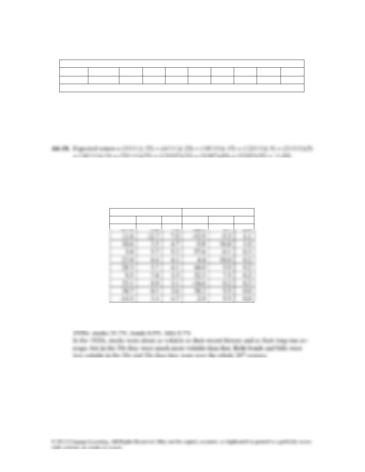
P6-19. Here are the nominal returns on stocks, bonds, and bills for the 1920s and 1930s. For each
decade, calculate the standard deviation of returns for each asset class. How do those fig-
ures compare with more recent numbers for stocks presented in Table 6.3 and the long-run
figures for all three asset types in Table 6.4?
Nominal Returns (%) on Stocks, Bonds, and Bills
1920s
1930s
Stocks
Bonds
Bills
Stocks
Bonds
Bills
A6-19. The standard deviations are as follows.
1920s: stocks 20.0%, bonds 3.4%, bills 1.5%
P6-20. Use the data below to calculate the standard deviation of nominal and real Treasury bill
returns from 1972-1982. Do you think that when they purchased T-bills investors expected
to earn negative real returns as often as they did during this period? If not, what happened
that took investors by surprise?
Chapter 6 The Trade-Off Between Risk and Return 173
Year
Nominal Return (%)
Real Return (%)
1972
3.8
0.4
1973
6.9
-1.7
1974
8.0
-3.7
1975
5.8
-1.1
1976
5.1
0.3
1977
5.1
-1.5
1978
7.2
-1.7
1979
10.4
-2.6
1980
11.2
-1.0
1981
14.7
5.3
1982
10.5
6.4
A6-20. The standard deviations are 3.3% in nominal terms and 3.2% in real terms. The negative
P6-21. Based on Figure 6.6, about what rate of return would a truly risk-free investment (i.e., one
with a standard deviation of zero) offer investors?
The Power of Diversification
P6-22. Troy McClain wants to form a portfolio of four different stocks. Summary data on the four
stocks follows. First calculate the average standard deviation across the four stocks, and
then answer this question: If Troy forms a portfolio by investing 25% of his money in each
of the stocks in the table, is it very likely that the standard deviation of this portfolios re-
turn will be (more than, less than, equal to) 43.5%?
Stock
Return
Standard
Deviation
1
14%
71%
2
10%
46%
3
9%
32%
4
11%
25%
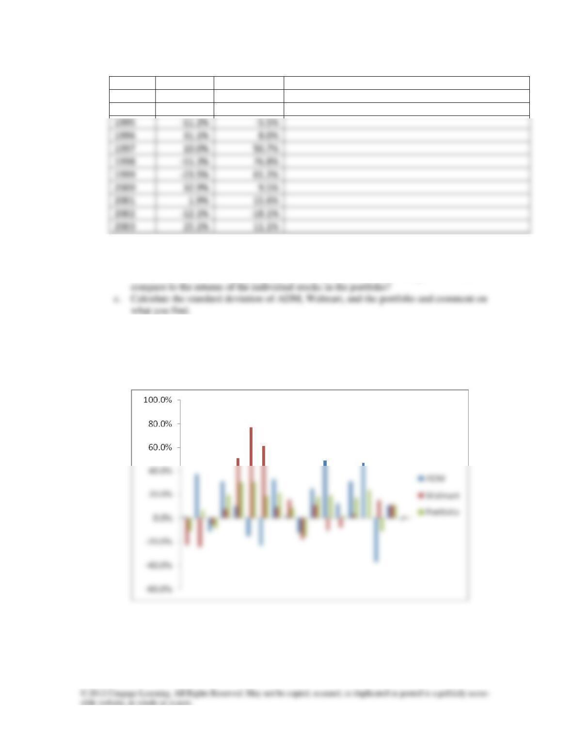
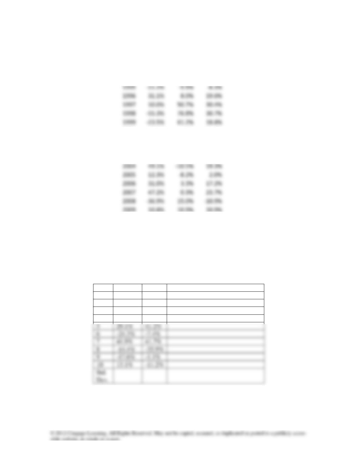
P6-23. The table below shows annual returns on Archer Daniels Midland (ADM) and Walmart
The last column of the table shows the annual return that a portfolio invested 50% in ADM
and 50% in Walmart would have earned in 1993. The portfolio’s return is simply a
weighted average of the returns of ADM and Walmart.
174 Instructor’s Manual
Year
AMD
Walmart
50-50 Portfolio
1993
1.5%
-22.7%
-10.6% = (0.5 X 1.5% + 0.5 X -22.7%)
1994
37.4%
-24.6%
1995
1996
31.1%
1997
10.0%
1998
1999
2000
32.9%
2001
1.9%
2002
–18.1%
2003
25.1%
a. Plot a graph similar to Figure 6.7 showing the returns on ADM and Walmart each year.
b. Fill in the blanks by calculating the 50-50 portfolio’s return each year from 1994-2010
and then plot this on the graph you created for part (a). How does the portfolio return
A6-23 a. The graph below shows returns each year on the two stocks and on the portfolio. In
general, the return on the portfolio each year falls between the returns on the stocks.
The standard deviation of the portfolio is much less than the standard deviation of ei-
ther stock in the portfolio.
Chapter 6 The Trade-Off Between Risk and Return 175
b. & c.
Year
ADM
Walmart
50–50
1993
1.5%
-22.7%
-10.6%
1994
37.4%
-24.6%
6.4%
1995
-11.2%
-8.3%
1996
31.1%
8.0%
19.6%
1997
10.0%
50.7%
30.4%
1998
-15.3%
76.8%
30.7%
1999
-23.5%
61.2%
18.8%
2000
32.9%
9.5%
21.2%
2001
1.9%
15.6%
8.7%
2002
-12.1%
-18.1%
-15.1%
2003
25.1%
11.1%
18.1%
2004
49.1%
-10.5%
19.3%
2005
12.3%
2.0%
2006
31.0%
3.3%
17.2%
2007
47.2%
0.3%
23.7%
2008
-36.9%
15.0%
-10.9%
2009
10.8%
10.9%
10.9%
2010
-1.5%
1.4%
0.0%
Std. dev
24.81%
27.71%
14.43%
P6-24. The table below shows annual returns for Merck and one of its major competitors, Eli
Lilly. The final column shows the annual return on a portfolio invested 50% in Lilly and
50% in Merck. The portfolio’s return is simply a weighted average of the returns of the
stocks in the portfolio as shown in the example calculation at the top of the table.
Year
Eli Lilly
Merck
50-50 Portfolio
1
15.4%
14.9%
15.1% (0.5 x 15.4% + 0.5 x 14.9%)
2
77.2%
76.4%
3
32.6%
24.0%
4
93.6%
35.5%
5
29.1%
41.2%
6
-24.3%
-7.4%
7
41.9%
41.7%
8
-14.4%
-35.9%
9
-17.6%
-1.1%
10
13.1%
-11.2%
a. Plot a graph similar to Figure 6.7 showing the returns on Merck and Lilly each year.
b. Fill in the blanks by calculating the 50-50 portfolio’s return each year from year 2 to
year 10, and then plot this on the graph you created for part (a). How does the portfo-
lio return compare to the returns of the individual stocks in the portfolio?
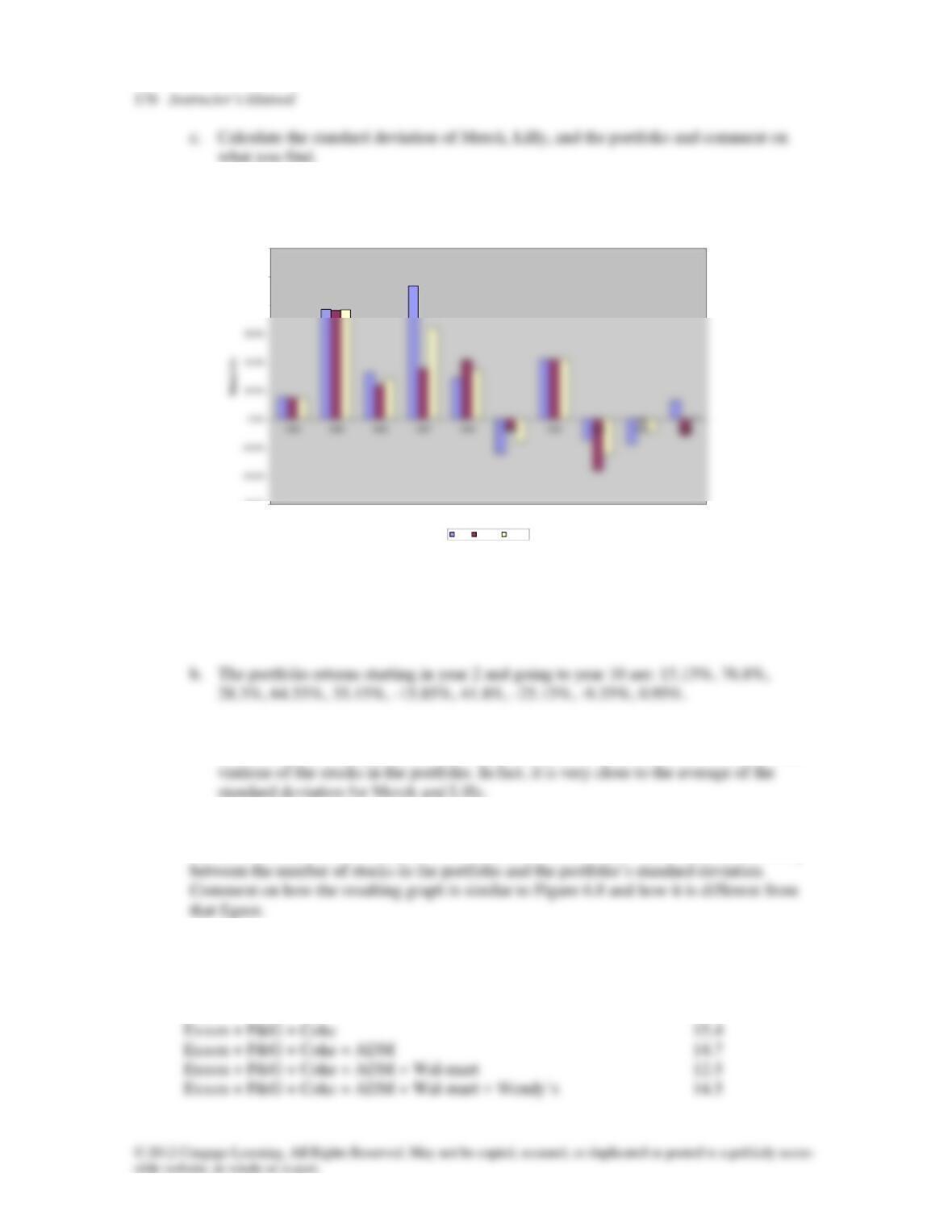
A6-24. a.
Annual Returns on Eli Lilly, Merck, and a 50-50 Portfolio
-60.0%
80.0%
100.0%
120.0%
Year
Lilly Merck 50-50
Notice how similar the return on Merck and Lilly are just about every year. This is not
too surprising because they operate in the same industry and are subject to many of the
same risks. A portfolio invested in these two stocks will provide much lower diversifi-
cation benefits than a portfolio invested in two companies in different industries (such
as Merck and AMD).
c. The standard deviations of Lilly, Merck, and the portfolio are 39.2%, 32.7%, and
34.2%. Notice that the portfolio’s standard deviation is very similar to the standard de-
P6-25. In this problem you will generate a graph similar to Figure 6.8. The table below shows the
standard deviation for various portfolios of stocks listed in Table 6.5. Plot the relationship
Stocks in the Portfolio
Std. Deviation
(%)
Exxon
16.6
Exxon + P&G
15.2
Exxon + P&G + Coke
15.4
Exxon + P&G + Coke + ADM
14.7
THOMSON ONE Business School Edition: Access financial information from the Thomson
create a username and password. Register your access serial number and then click Enter on the
aforementioned Web site. When you click Enter, you will be prompted for your username and
password (please remember that the password is case sensitive). Enter them in the respective boxes
and then click OK (or hit Enter). From the ensuing page, click Click Here to Access Thomson
ONE – Business School Edition Now! This opens up a new window that gives you access to the
Thomson ONE – Business School Edition database. You can retrieve a company’s financial infor-
mation by entering its ticker symbol (provided for each company in the problem[s]) in the box be-
low “Name/Symbol/Key.”
Answer to MiniCase
The Trade-Off Between Risk and Return
Assignment
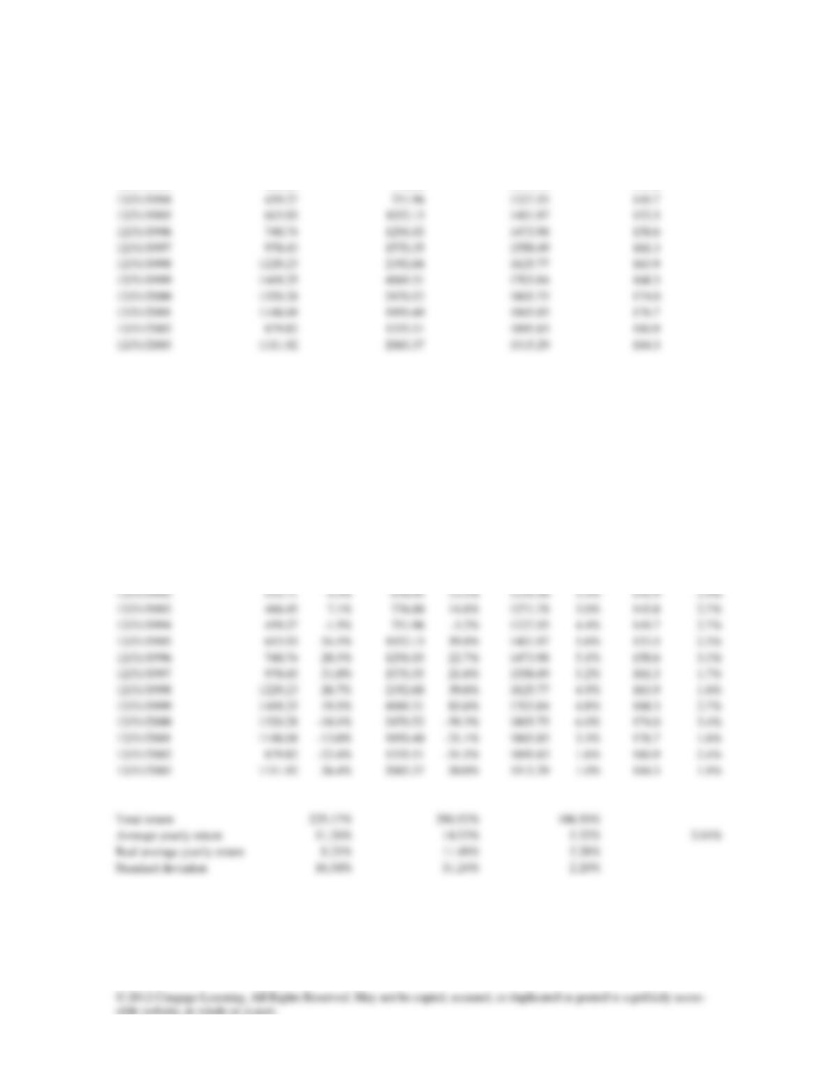
Use the following information to compare the recent performance of the S&P 500 Index, the
Nasdaq Index, and the Treasury Bill Index from 1983-2003. Each of these index numbers is calcu-
lated in a way that assumes that investors reinvest any income they receive, so the total return
equals the percentage change in the index value each year. The last column shows the level of the
the standard deviation of each asset class on the horizontal axis and the average return on the
vertical axis.
Date S&P 500 Nasdaq T-Bills CPI
12/31/1983 164.93 278.60 681.44 101.3
12/31/1984 167.24 247.35 748.88 105.3
12/31/1988 277.72 381.38 968.89 120.5
178 Instructor’s Manual
12/31/1989 353.40 454.82 1050.63 126.1
12/31/1990 330.22 373.84 1131.42 133.8
12/31/1991 417.09 586.34 1192.83 137.9
12/31/1992 435.71 676.95 1234.36 141.9
12/31/1993 466.45 776.80 1271.78 145.8
Answer:
Date S&P 500 NASDAQ T-Bills CPI
12/31/1983 164.93 278.60 681.44 101.3
12/31/1984 167.24 1.4% 247.35 -11.2% 748.88 9.9% 105.3 3.9%
12/31/1985 211.28 26.3% 324.39 31.1% 806.62 7.7% 109.3 3.8%
12/31/1986 242.17 14.6% 348.81 7.5% 855.73 6.1% 110.5 1.1%
12/31/1987 247.08 2.0% 330.47 -5.3% 906.02 5.9% 115.4 4.4%
12/31/1988 277.72 12.4% 381.38 15.4% 968.89 6.9% 120.5 4.4%
12/31/1989 353.40 27.3% 454.82 19.3% 1050.63 8.4% 126.1 4.6%
12/31/1990 330.22 -6.6% 586.34 -17.8% 1131.42 7.7% 133.8 6.1%
12/31/1991 417.09 26.3% 586.34 56.8% 1192.83 5.4% 137.9 3.1%
A positive relation between average return and standard deviation obtains in these figures.
NASDAQ earned the highest average returns, but had the highest volatility as well. T-bills varied
the least, but they earned the lowest returns.