1
2
3
4
5
6
7
8
9
10
11
12
13
14
15
16
17
18
19
consulting with the economists at your firm, you have specified 5 possible scenarios for the resolution of the
dispute at the end of the year. For each scenario, you have estimated the probability of the scenario occurring
and the impact on interest rates and bond prices if the scenario occurs. Given this information, you have
calculated the rate of return on 10-year zero coupon Treasury bonds for each scenario. The probabilities and
returns are shown further below.
20
21
22
23
24
25
26
27
28
29
30
31
32
33
34
35
36
37
38
39
40
41
42
43
44
45
46
Poor Case 0.20 −4%
Most Likely 0.40 6%
Good Case 0.20 16%
49
50
51
52
53
54
55
56
57
58
59
60
61
62
63
64
65
66
67
68
69
70
71
72
73
74
A B C D E F G H I J
11/20/2018
Amount invested $1,000
Amount received in one year $1,060
Dollar return (Profit) $60
Rate of return = Profit/Investment = 6%
Worst Case 0.10 −14%
Return on a 10-
Year Zero
Coupon
Treasury Bond
During Next
Year
Probability of
Scenario
Discrete Probability Distribution for 5 Scenarios
CHAPTER 6 MINI CASE
a. What are investment returns? What is the return on an investment that costs $1,000 and is sold after 1 year
for $1,060?
b. Graph the probability distribution for the 5 scenarios during the next year for the 10-year zero coupon bonds.
What might the graph of the probability distribution look like if there were an infinite number of scenarios (i.e.,
if it were a continuous distribution and not a discrete distribution)?
You have also gathered historical returns for the past 10 years for Blandy, Gourmange Corporation (a producer
of gourmet specialty foods), and the stock market.
The risk-free rate is 4% and the market risk premium is 5%.
Assume that you recently graduated and landed a job as a financial planner with Cicero Services, an investment
advisory company. Your first client recently inherited some assets and has asked you to evaluate them. The
client presently owns a bond portfolio with $1 million invested in zero coupon Treasury bonds that mature in 10
years. The client also has $2 million invested in the stock of Blandy, Inc., a company that produces meat-and-
potatoes frozen dinners. Blandy’s slogan is “Solid food for shaky times.”
Scenario
0.20
0.25
0.30
0.35
0.40
0.45
Probability of
Scenario
75
76
77
78
79
80
81
82
83
84
85
86
87
88
89
90
91
92
93
94
95
96
97
98
99
100
101
102
103
104
105
106
107
108
111
Most Likely 0.40 6% 2.4%
Good Case 0.20 16% 3.2%
112
113
114
115
116
117
118
119
120
121
122
123
124
125
126
129
130
131
132
133
134
135
136
137
Poor Case 0.20 −4% −0.8% −10% 1.0% 0.2%
Most Likely 0.40 6% 2.4% 0% 0.0% 0.0%
Good Case 0.20 16% 3.2% 10% 1.0% 0.2%
Excel functions for finding expected return and standard deviation of discrete events
Use SUMPRODUCT to find expected return by putting probabilities in first argument array and
rates of return in the second argument array.
Use SUMPRODUCT to find variance by putting probabilities in first argument array and the
outcomes minus the expected value in the second and third arrays.
Take the square root of the variance to get the standard deviation.
138
139
140
141
142
143
144
145
A B C D E F G H I J
Calculating Expected Returns
Inputs: Expected Return
Scenario
Probability of
Scenario
(1)
Rate of Return
(2)
Product of
Probability and
Return
(1) x (2) = (3)
Worst Case 0.10 −14% −1.4%
Poor Case 0.20 −4% −0.8%
Excel function for finding expected return of discrete events:
Calculating Expected Returns and Standard Deviations: Discrete Probabilities
Inputs: Expected Return
Scenario
Probability of
Scenario
(1)
Rate of Return
(2)
Product of
Probability and
Return
(1) x (2) = (3)
Deviation from
Expected Return
(2) − Exp. r = (4)
Squared
Deviation
(4)2 = (5)
Sq. Dev. ×
Prob.
(1) x (5) = (6)
Worst Case 0.10 −14% −1.4% −20% 4.0% 0.4%
Use SUMPRODUCT to find expected return by putting probabilities in first argument array and
rates of return in the second argument array.
d. What is stand-alone risk? Use the scenario data to calculate the standard deviation of the bond’s return for the
next year.
Standard Deviation
c. Use the scenario data to calculate the expected rate of return for the 10-year zero coupon Treasury bonds
during the next year.
6%
e. Your client has decided that the risk of the bond portfolio is acceptable and wishes to leave it as it is. Now your
client has asked you to use historical returns to estimate the standard deviation of Blandy’s stock returns. (Note:
Many analysts use 4 to 5 years of monthly returns to estimate risk and many use 52 weeks of weekly returns;
some even use a year or less of daily returns. For the sake of simplicity, use Blandy’s 10 annual returns.)
0.10
0.12
0.14
0.16
0.18
Probability
Continuous Probability Distribution
146
147
148
149
150
160
161
162
163
164
165
166
167
168
169
170
171
172
173
174
175
176
177
178
188
189
190
191
192
193
194
195
196
197
198
199
200
201
202
203
204
A B C D E F G H I J
Year Market Blandy Gourmange
130% 26% 47%
27% 15% -54%
318% -14% 15%
Blandy Gourmange
Weight in : 75% 25%
Year Blandy Gourmange Portfolio
126% 47% 31.3%
215% -54% -2.3%
3 -14% 15% -6.8%
Notice that the historical returns for Blandy and Gourmange do not move in perfect lockstep.
f. Your client is shocked at how much risk Blandy stock has and would like to reduce the level of risk. You suggest
that the client sell 25% of the Blandy stock and create a portfolio with 75% Blandy stock and 25% in the high-
risk Gourmange stock. How do you suppose the client will react to replacing some of the Blandy stock with high-
risk stock? Show the client what the proposed portfolio return would have been in each year of the sample. Then
calculate the average return and standard deviation using the portfolio’s annual returns. How does the risk of
this two-stock portfolio compare with the risk of the individual stocks if they were held in isolation?
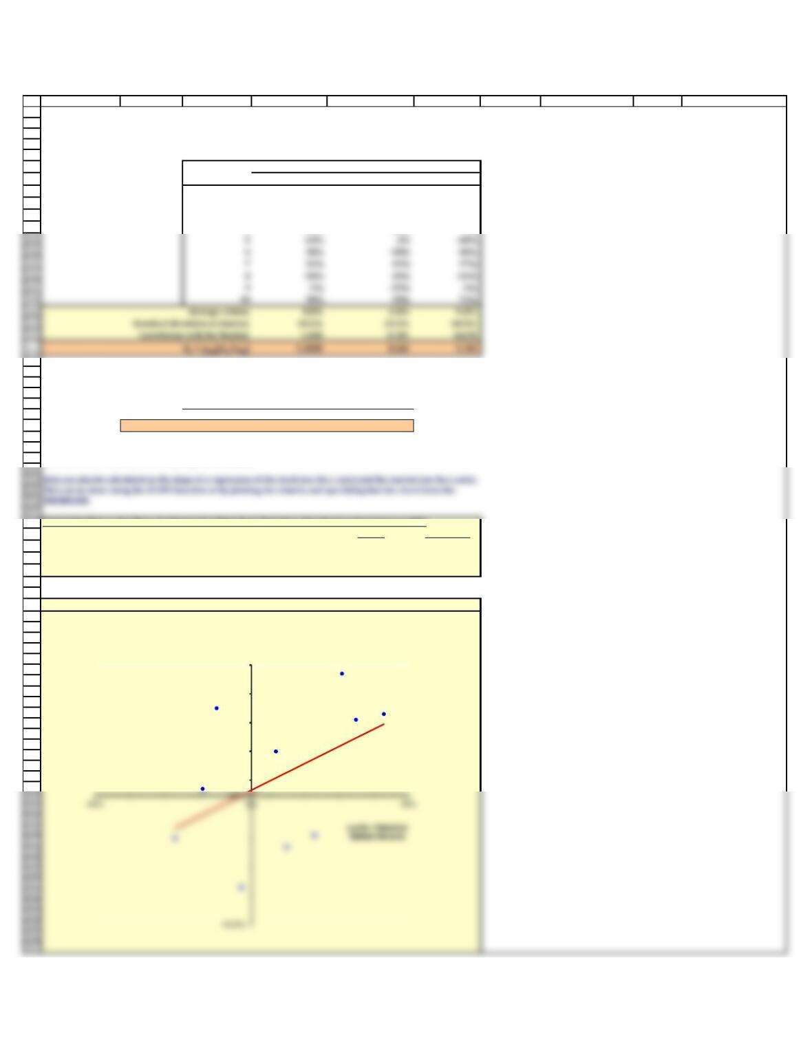
Stock Returns
g. Explain correlation to your client. Calculate the estimated correlation between Blandy and Gourmange. Does
this explain why the portfolio standard deviation was less than Blandy’s standard deviation?
Historical Stock Returns for Blandy and Gourmange
Stock Returns
Gourmange
30%
45%
60%
75%
Rate of Return
216
217
218
219
220
221
222
223
224
225
226
227
228
229
230
231
232
233
234
235
236
237
238
239
240
241
242
243
244
245
246
247
248
249
250
251
252
253
254
255
256
257
258
259
260
261
262
263
264
265
266
267
268
269
270
271
272
273
274
275
276
277
279
280
281
282
284
285
286
287
289
290
291
The SML predicts stock i’s required return to be:
A B C D E F G H I J
Correlation between Blandy and Gourmange
r = 0.11 Use the Excel function: =CORREL(Blandy_returns,Gourmange_returns)
Beta for Stock i = bi = riM(si/sM)
rRF The risk-free rate. It varies over time, but is constant for all firms at a given time.
i. (1.) Should portfolio effects impact the way investors think about the risk of individual stocks? Answer: See Ch
06 Mini Case Show
(2.) If you decided to hold a 1-stock portfolio and consequently were exposed to more risk than diversified
investors, could you expect to be compensated for all of your risk; that is, could you earn a risk premium on that
part of your risk that you could have eliminated by diversifying? Answer: See Ch 06 Mini Case Show
The relevant risk of an individual stock as defined by its beta. Beta measures how much standard deviation a
stock contributes to the standard deviation of a well-diversified portfolio.
Loosely speaking, correlation measures the tendency of two variables to move together.
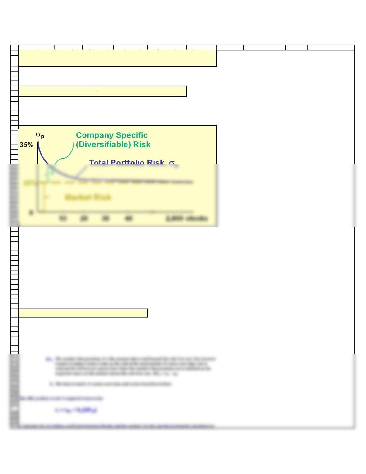
h. Suppose an investor starts with a portfolio consisting of one randomly selected stock. As more and more
randomly selected stocks are added to the portfolio, what happens to the portfolio’s risk?
given) standard deviations of Blandy and the market to estimate Blandy’s beta. Does Blandy contribute more or
less risk to a well-diversified portfolio than does the average stock? Use the SML to estimate Blandy’s required
return. Assume that the risk-free rate is 4% and the market risk premium is 5%. Use the SML to estimate
Blandy’s required return.
k. What is the Security Market Line? How is beta related to a stock’s required rate of return?
The SML shows the relationship between the stock’s beta and its required return, as predicted by the CAPM.
j. According to the Capital Asset Pricing model, what measures the amount of risk that an individual stock
contributes to a well-diversified portfolio? Define this measurement.
-75%
1 2 3 4 5 6 7 8 9 10
Year
292
293
294
295
296
297
298
299
300
301
311
313
314
315
316
317
318
319
320
321
322
323
324
325
326
327
328
329
330
331
332
333
334
335
336
337
338
339
340
341
342
343
344
345
346
347
348
349
350
351
352
353
354
355
356
357
358
359
360
361
362
363
364
365
366
367
A B C D E F G H I J
Year Market Blandy Gourmange
130% 26% 47%
27% 15% -54%
318% -14% 15%
Risk-free rate = 4%
Market risk premium = 5%
Blandy Gourmange Average Stock
Beta = 0.60 1.30 1.00
ri = 7.0% 10.5% 9.0%
Blandy Gourmange
bi = riM(si/sM)0.603 1.301 =SLOPE(y_values,x_values)
Intercept 0.016 -0.012 =INTERCEPT(y_values,x_values)
R squared 0.232 0.460 =RSQ(y_values,x_values)
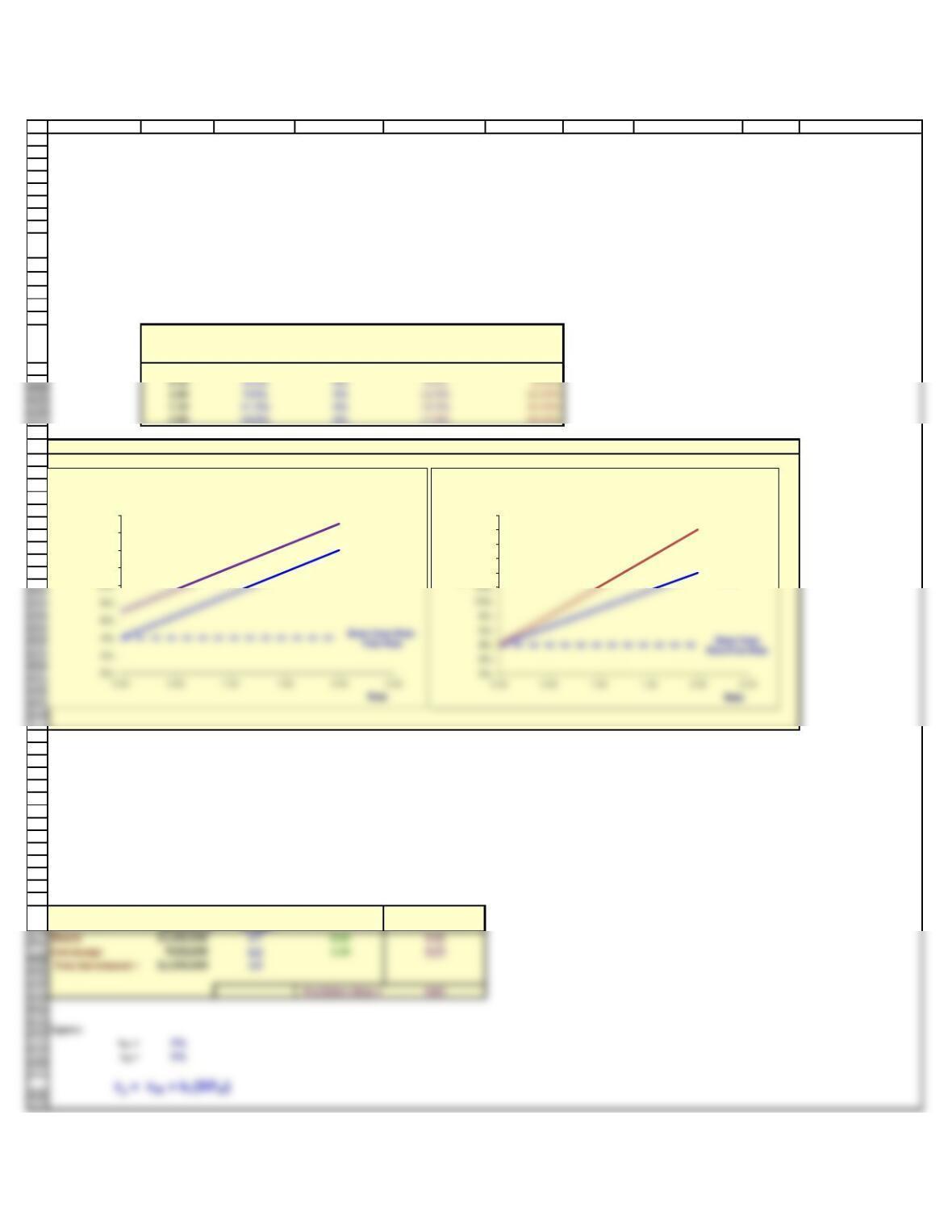
Calculating Beta as the Slope of a Regression Using Excel Functions (See Excel explanations to right)
Stock Returns
l. Calculate the correlation coefficient between Blandy and the market. Use this and the previously calculated (or
given) standard deviations of Blandy and the market to estimate Blandy’s beta. Does Blandy contribute more or
less risk to a well-diversified portfolio than does the average stock? Use the SML to estimate Blandy’s required
return. Assume that the risk-free rate is 4% and the market risk premium is 5%. Use the SML to estimate
Blandy’s required return.
m. Show how to estimate beta using regression analysis.
Stock Returns of Blandy and the Market: Estimating Beta
y = 0.6027x + 0.0158
R² = 0.2316
45.0%
y-axis: Historical
Blandy Returns
368
369
370
371
372
373
374
375
376
377
378
379
380
381
382
383
384
385
386
387
0.50 6.5% 4% 9.5% 8.00%
1.00 9.0% 4% 12.0% 12.00%
388
389
390
391
392
393
394
395
396
397
398
399
400
401
402
403
404
405
406
407
408
409
410
411
412
413
414
415
416
417
418
419
420
421
422
423
424
425
427
429
430
431
432
433
434
437
439
A B C D E F G H I J
Base Case
Higher Risk-
Free Rate
Higher Market
Risk Premium
rRF 4% 7% 4%
rM5% 5% 8%
Beta
SML: Base Case
Base Case Risk-
Free Rate
SML: Higher Risk-
Free Rate
SML: Higher
Market Risk
Premium
0.00 4.0% 4% 7.0% 4.00%
Stock
Amount of
Portfolio
Beta Weighted Beta
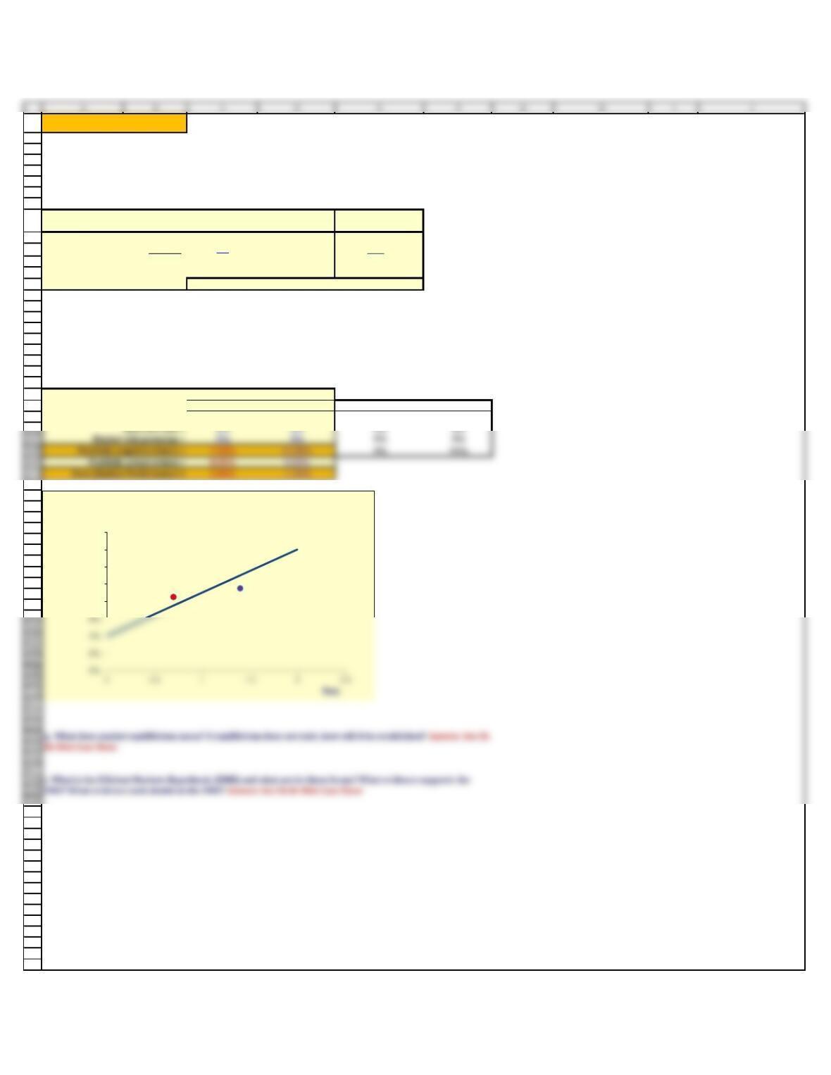
Changes to Inputs for the Security Market Line
The Security Market Line shows the projected changes in expected return, due to changes in the beta coefficient.
However, we can also look at the potential changes in the required return due to variations in other factors, for
example the market return and risk-free rate. In other words, we can see how required returns can be
influenced by changing inflation and risk aversion. The level of investor risk aversion is measured by the market
risk premium (rM – rRF), which is also the slope of the SML. Hence, an increase in the market return results in an
increase in the maturity risk premium, other things held constant.
n. (1) Suppose interest rates go up by 3 percentage points over the current 4% risk-free rate. What effect would
higher interest rates have on the SML and on the returns required on high- and low-risk securities? (2) Suppose
instead that investors’ risk aversion increased enough to cause the market risk premium to increase by 3
percentage points. (Assume the risk-free rate remains constant.) What effect would this have on the SML and on
returns of high- and low-risk securities?
o. Your client decides to invest $1.4 million in Blandy stock and $0.6 million in Gourmange stock. What are the
weights for this portfolio? What is the portfolio’s beta? What is the required return for this portfolio?
SML: Base Case
SML: Higher
Risk-Free Rate
12%
14%
16%
18%
Required Return
Impact of Increase in Risk-Free Rate
SML: Base
Case
SML: Higher
Market Risk
Premium
14%
16%
18%
20%
22%
Required Return
Impact of Increase in Market Risk Premium
440
441
442
443
444
445
446
447
448
449
450
451
452
453
454
455
456
457
458
459
460
461
462
463
464
465
466
467
468
469
470
Risk-free rate = 4% 4% 4% 4%
471
472
473
474
475
476
477
478
479
480
481
482
483
484
485
486
487
488
489
490
491
492
493
494
495
496
497
498
500
501
502
503
504
505
506
507
508
509
510
511
512
513
514
515
rp = 8.06%
Alternative Approach to Find Required Return on Porfolio
Stock
Amount of
Investment
Portfolio
Weight
Required Return Weighted Return
Blandy $1,400,000 0.7 7.0% 4.91%
Gourmange $600,000 0.3 10.5% 3.15%
Total investment = $2,000,000 1.0
Portfolio’s Return = 8.06%
JJ CC
Portfolio beta = 0.7 1.4 0 2
The required return on a portfolio is a weighted average of the required returns of the individual assets in the
portfolio.
Portfolio Manager
Additonal data for graph
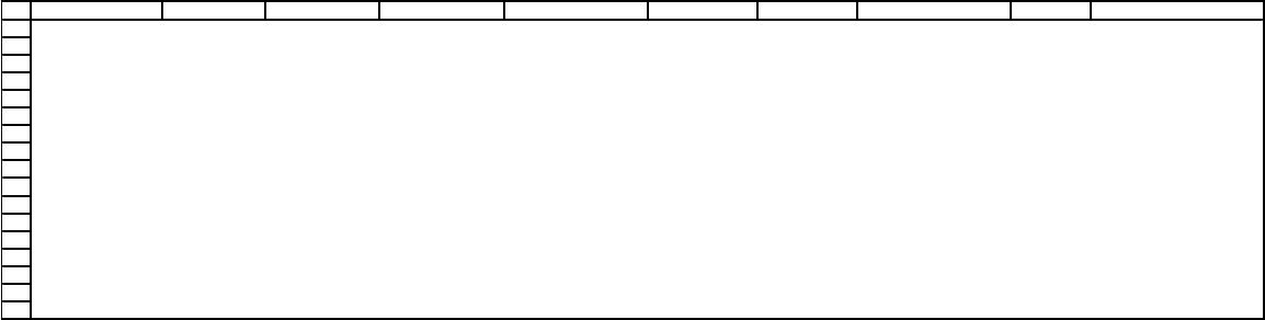
p. Jordan Jones (JJ) and Casey Carter (CC) are portfolio managers at your firm. Each manages a well-diversified
portfolio. Your boss has asked for your opinion regarding their performance in the past year. JJ’s portfolio has a
beta of 0.6 and had a return of 8.5%; CC’s portfolio has a beta of 1.4 and had a return of 9.5%. Which manager
had better performance? Why?
SML
JJ-Actual CC-Actual
8%
10%
12%
14%
16%
Required Return
Performance Evaluation
516
517
518
519
520
521
522
523
524
525
526
527
528
529
530
531
532
A B C D E F G H I J

533
534
535
536
537
538
539
540
541
542
543
544
545
546
547
548
549
550
551
552
553
554
555
556
557
558
559
560
561
562
563
564
565
A B C D E F G H I J