Chapter 6
Risk and Return
ANSWERS TO END-OF-CHAPTER QUESTIONS
6-1 a. Stand-alone risk is only a part of total risk and pertains to the risk an investor takes by
holding only one asset. Risk is the chance that some unfavorable event will occur. For
instance, the risk of an asset is essentially the chance that the asset’s cash flows will be
unfavorable or less than expected. A probability distribution is a listing, chart or graph
of all possible outcomes, such as expected rates of return, with a probability assigned
to each outcome. When in graph form, the tighter the probability distribution, the less
uncertain the outcome.
d. The standard deviation (σ) is a statistical measure of the variability of a set of
observations. The variance (σ2) of the probability distribution is the sum of the squared
deviations about the expected value adjusted for deviation.
e. A risk averse investor dislikes risk and requires a higher rate of return as an inducement
to buy riskier securities. A realized return is the actual return an investor receives on
their investment. It can be quite different than their expected return.
h. The expected return on a portfolio.
r
p, is simply the weighted-average expected return
of the individual stocks in the portfolio, with the weights being the fraction of total
portfolio value invested in each stock. The market portfolio is a portfolio consisting of
all stocks.
j. Market risk is that part of a security’s total risk that cannot be eliminated by
diversification. It is measured by the beta coefficient. Diversifiable risk is also known
as company specific risk, that part of a security’s total risk associated with random
events not affecting the market as a whole. This risk can be eliminated by proper
diversification. The relevant risk of a stock is its contribution to the riskiness of a well-
diversified portfolio.
l. The security market line (SML) represents in a graphical form, the relationship between
the risk of an asset as measured by its beta and the required rates of return for individual
securities. The SML equation is essentially the CAPM, ri = rRF + bi(RPM). It can also
be written in terms of the required market return: ri = rRF + bi(rM – rRF).
n. Equilibrium is the condition under which the expected return on a security is just equal
to its required return,
r
= r, and the market price is equal to the intrinsic value. The
Efficient Markets Hypothesis (EMH) states (1) that stocks are always in equilibrium
and (2) that it is impossible for an investor to consistently “beat the market.” In essence,
the theory holds that the price of a stock will adjust almost immediately in response to
any new developments. In other words, the EMH assumes that all important
information regarding a stock is reflected in the price of that stock. Financial theorists
generally define three forms of market efficiency: weak-form, semistrong-form, and
o. The Fama-French 3-factor model has one factor for the excess market return (the
market return minus the risk free rate), a second factor for size (defined as the return
on a portfolio of small firms minus the return on a portfolio of big firms), and a third
factor for the book–to-market effect (defined as the return on a portfolio of firms with
a high book-to-market ratio minus the return on a portfolio of firms with a low book–
to-market ratio).
6-2 a. The probability distribution for complete certainty is a vertical line.
b. The probability distribution for total uncertainty is the X axis from – to +.
6-4 The risk premium on a high beta stock would increase more.
RPj = Risk Premium for Stock j = (rM – rRF)bj.
If risk aversion increases, the slope of the SML will increase, and so will the market risk
premium (rM – rRF). The product (rM – rRF)bj is the risk premium of the jth stock. If bj is
low (say, 0.5), then the product will be small; RPj will increase by only half the increase in
RPM. However, if bj is large (say, 2.0), then its risk premium will rise by twice the increase
in RPM.
SOLUTIONS TO END-OF-CHAPTER PROBLEMS
6-1 Investment Beta
$20,000 0.7
35,000 1.3
Total $55,000
($20,000/$55,000)(0.7) + ($35,000/$55,000)(1.3) = 1.08.
6-3 rRF = 5%; RPM = 7%; rM = ?
rM = 5% + (7%)1 = 12% = rs when b = 1.0.
rs when b = 1.7 = ?
rs = 5% + 7%(1.7) = 16.9%.
6-4 Predicted return = ai + bi(r¯ M,t) + ci(r¯ SMB,t) + di(r¯ HML,t)
= 0.0% + 1.2(10%) + (-0.4)(3.2%) + 1.3(4.8%)
= 16.96%
6-7 a. rA = rRF + (rM – rRF)bA
12% = 5% + (10% – 5%)bA
12% = 5% + 5%(bA)
7% = 5%(bA)
1.4 = bA.
6-8 a. ri = rRF + (rM – rRF)bi = 5% + (12% – 5%)1.4 = 14.8%.
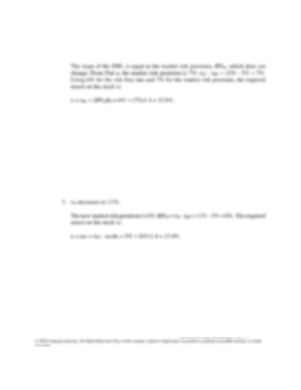
b. 1. rRF increases to 6%:
2. rRF decreases to 4%:
ri = rRF + (RPM)bi = 4% + (7%)1.4 = 13.8%.
c. 1. rM increases to 14%:
If the risk-free rate does not change but they required return on the market does
change, then the market risk premium changes. For rRF = 5% and rM = 14%, the
new market risk premium is 9%: RPM = rM – rRF = 14% – 5% = 9%. The required
return on the stock is:
ri = rRF + (RPM)bi = 5% + (9%)1.4 = 17.6%.
6-9 Old portfolio beta =
5,0007$
000,70$
(b) +
5,0007$
000,5$
(0.8)
Alternative Solutions:
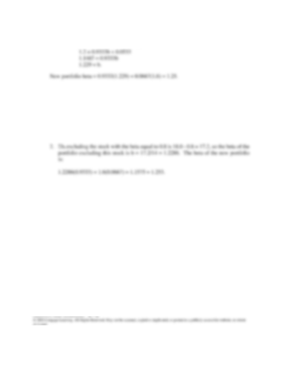
1. Old portfolio beta = 1.2 = (0.0667)b1 + (0.0667)b2 +…+ (0.0667)b20
1.2 = (bi)(0.0667)
bi = 1.2/0.0667 = 18.0.
New portfolio beta = (18.0 – 0.8 + 1.6)(0.0667) = 1.253 = 1.25.
6-10 Portfolio beta =
$4,000,000
$400,000
(1.50) +
$4,000,000
$600,000
(-0.50)
+
$4,000,000
$4,000,000
$1,000,000
(1.25) +
$2,000,000
(0.75)
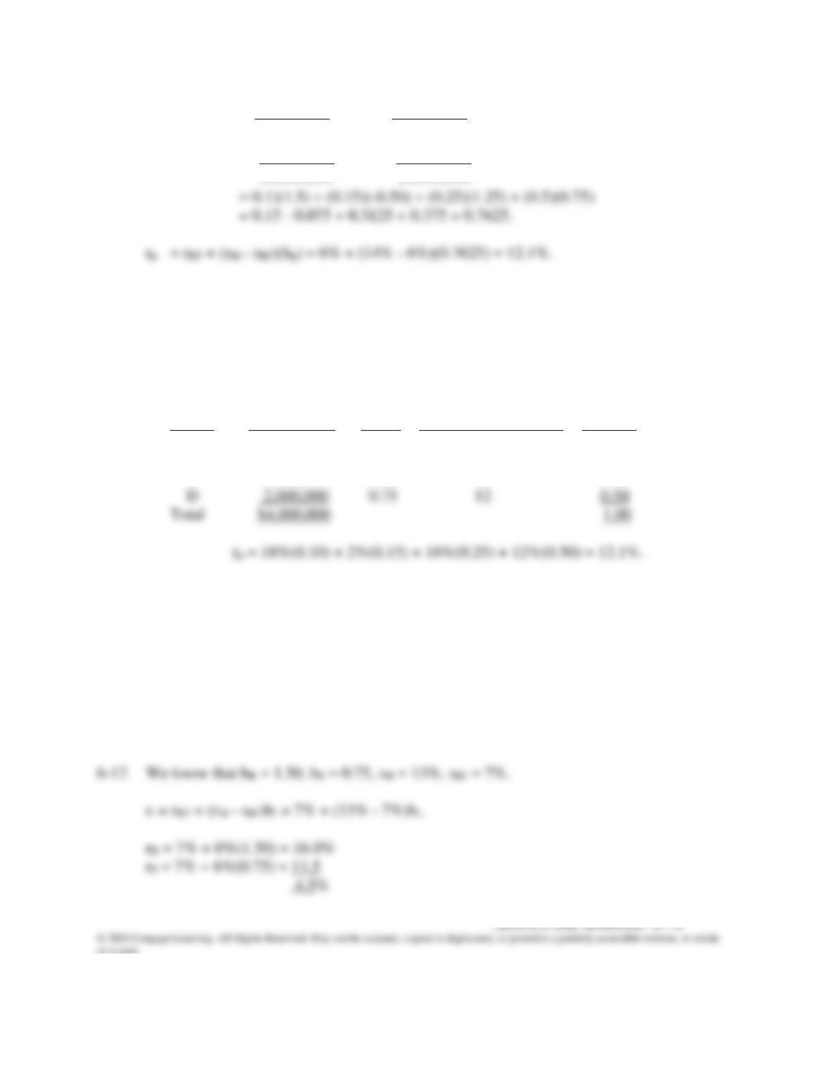
Alternative solution: First compute the return for each stock using the CAPM equation
[rRF + (rM – rRF)b], and then compute the weighted average of these returns.
rRF = 6% and rM – rRF = 8%.
Stock Investment Beta r = rRF + (rM – rRF)b Weight
A $ 400,000 1.50 18% 0.10
B 600,000 (0.50) 2 0.15
C 1,000,000 1.25 16 0.25
6-11 First, calculate the beta of what remains after selling the stock:
bp = 1.1 = ($100,000/$2,000,000)0.9 + ($1,900,000/$2,000,000)bR
1.1 = 0.045 + (0.95)bR
bR = 1.1105.
bN = (0.95)1.1105 + (0.05)1.4 = 1.125.
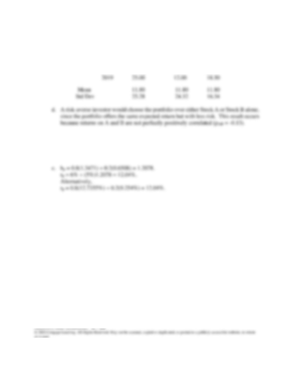
6-13 The answers to a, b, and c are given below:
¯rA ¯rB Portfolio
2015 (20.00%) (5.00%) (12.50%)
2016 42.00 15.00 28.50
2017 20.00 (13.00) 3.50
2018 (8.00) 50.00 21.00
6-14 a. bX = 1.3471; bY = 0.6508. These can be calculated with a spreadsheet.
b. rX = 6% + (5%)1.3471 = 12.7355%.
rY = 6% + (5%)0.6508 = 9.2540%.
SOLUTION TO SPREADSHEET PROBLEM
6-15 The detailed solution for the spreadsheet problem is available in the file Ch06-P15 Build
a Model Solution.xlsx on the textbook’s Web site.
Assume that you recently graduated and landed a job as a financial planner with Cicero
Services, an investment advisory company. Your first client recently inherited some assets
and has asked you to evaluate them. The client owns a bond portfolio with $1 million invested
in zero coupon Treasury bonds that mature in 10 years. The client also has $2 million
invested in the stock of Blandy, Inc., a company that produces meat-and-potatoes frozen
dinners. Blandy’s slogan is “Solid food for shaky times.”
Unfortunately, Congress and the president are engaged in an acrimonious dispute over the budget
rates and bond prices if the scenario occurs. Given this information, you have calculated the rate
of return on 10-year zero coupon Treasury bonds for each scenario. The probabilities and returns
are shown below:
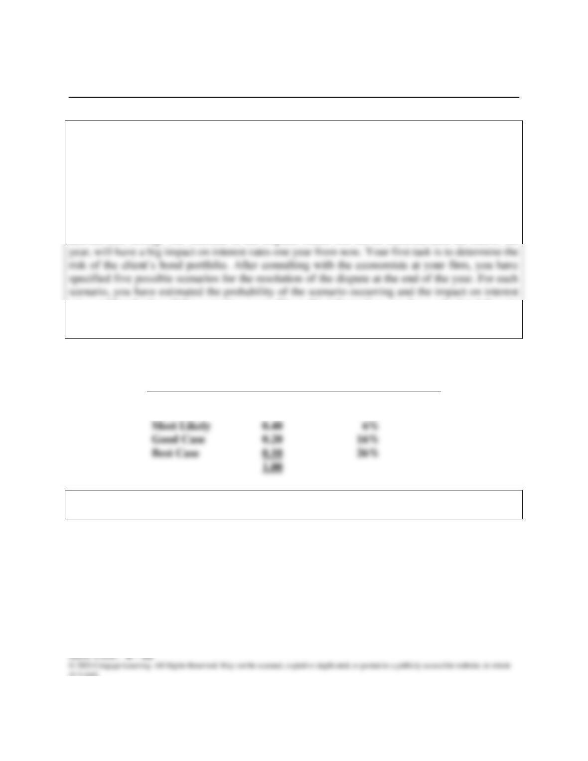
Scenario
Probability
of Scenario
Return on a 10-Year Zero
Coupon Treasury Bond
During the Next Year
Worst Case
0.10
−14%
Poor Case
0.20
−4%
Most Likely
0.40
Good Case
0.20
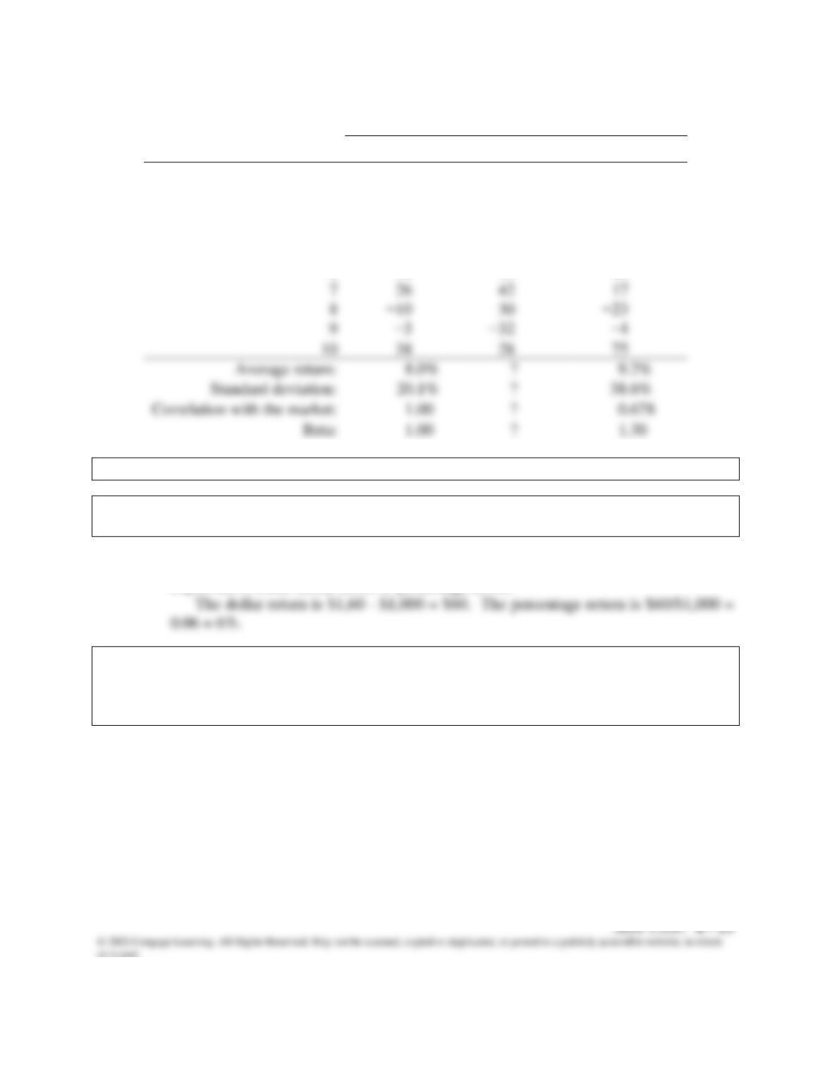
You have also gathered historical returns for the past 10 years for Blandy, Gourmange
Corporation (a producer of gourmet specialty foods), and the stock market.
MINI CASE
Historical Stock Returns
Year
Market
Blandy
Gourmange
1
30%
26%
47%
2
7
15
−54
3
18
−14
15
4
−22
−15
7
5
−14
2
−28
6
10
−18
40
7
26
42
17
8
−10
30
−23
9
−32
38
28
75
Average return:
The risk-free rate is 4% and the market risk premium is 5%.
a. What are investment returns? What is the return on an investment that costs
$1,000 and is sold after 1 year for $1,060?
Answer: Investment return measures the financial results of an investment. They may be
b. Graph the probability distribution for the bond returns based on the 5 scenarios.
What might the graph of the probability distribution look like if there were an
infinite number of scenarios (i.e., if it were a continuous distribution and not a
discrete distribution)?
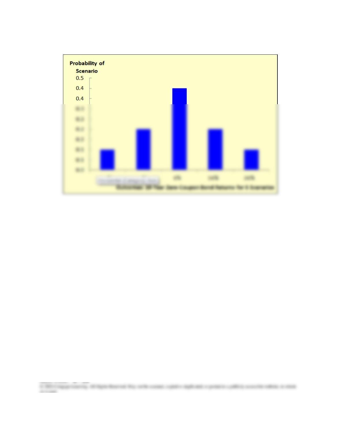
Answer: Here is the probability distribution for the five possible outcomes:
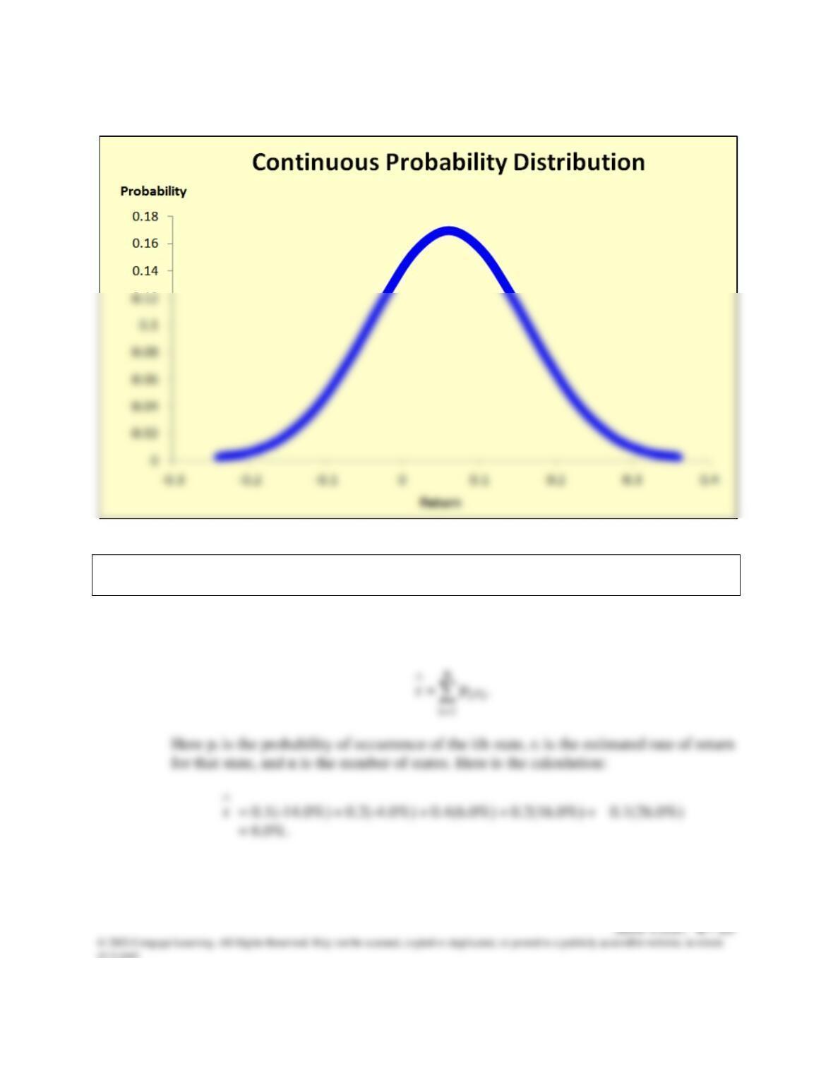
A continuous distribution might look like this:
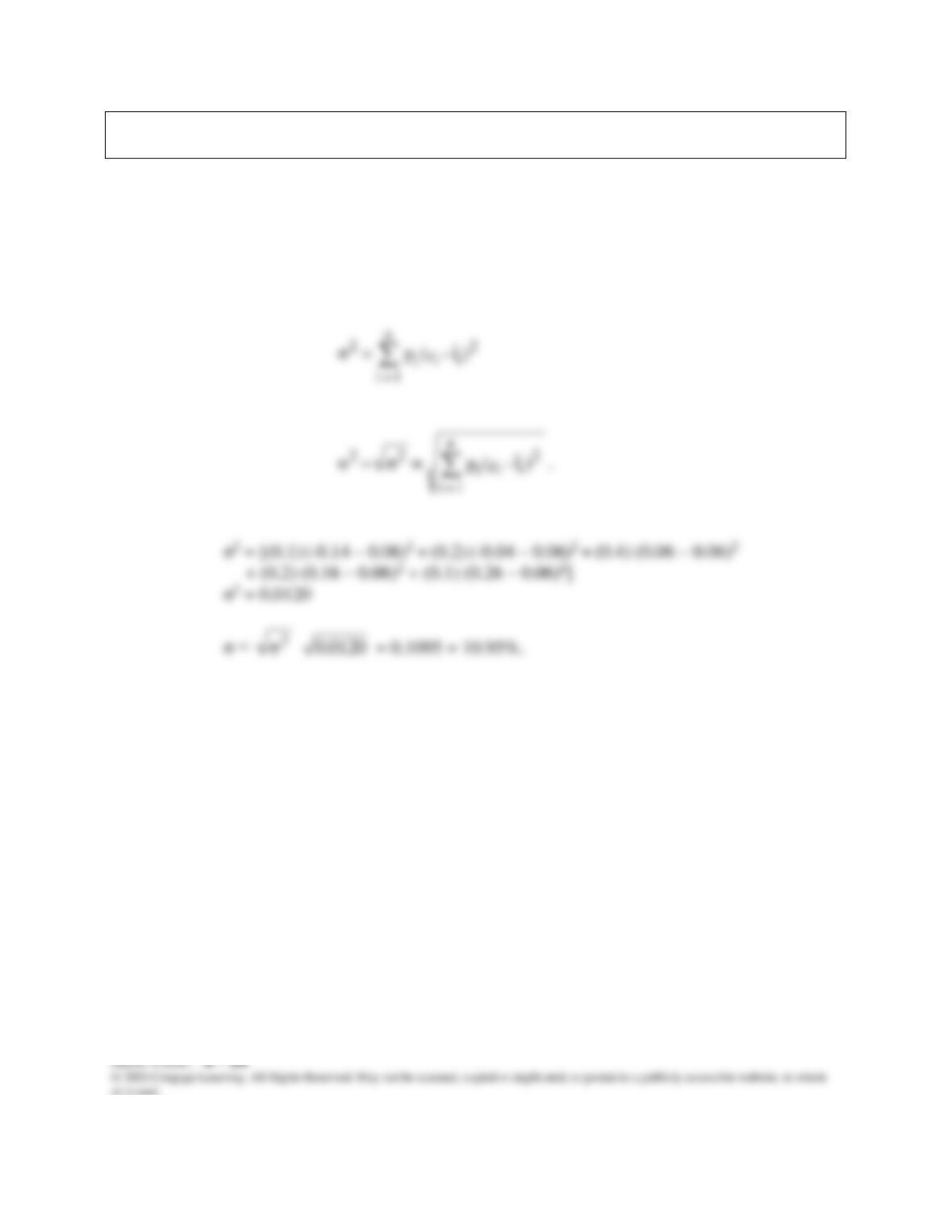
c. Use the scenario data to calculate the expected rate of return for the 10-year zero
coupon Treasury bonds during the next year.
Answer: The expected rate of return,
r
, is expressed as follows:
r
d. What is stand-alone risk? Use the scenario data to calculate the standard deviation
of the bond’s return for the next year.
Answer: Stand-alone risk is the risk of an asset if it is held by itself and not as a part of a portfolio.
Standard deviation measures the dispersion of possible outcomes, and for a single asset,
the stand-alone risk is measured by standard deviation.
The variance and standard deviation are calculated as follows: