1
2
3
4
5
6
7
8
9
15
16
17
18
31
Real risk free rate 2.0%
Expected inflation Year
Maturity risk premium Annual 2.0%
19
20
21
A B C D E F G H I
Chapter 5 Spreadsheet Problem Solutions (C05)
1. There are a number of instructions with which you should be familiar
to use these computerized models. These instructions appear in a
separate worksheet labeled INSTRUCTIONS. If you have not already
done so, you should read these instructions now. To read these
instructions, click on theworksheet labeled INSTRUCTIONS.
3. Graphs that show the yield curves will be displayed when you click on
the worksheets labeled “Yield Curve” and “Corporate.”
INPUT DATA:
Current year (end of year) 0
Yield Curve
2. The input data are entered in specified cells in the INPUT DATA
section. When you change an input item, the model automatically
recalculates the values of appropriate output data items, unless
you are told otherwise.

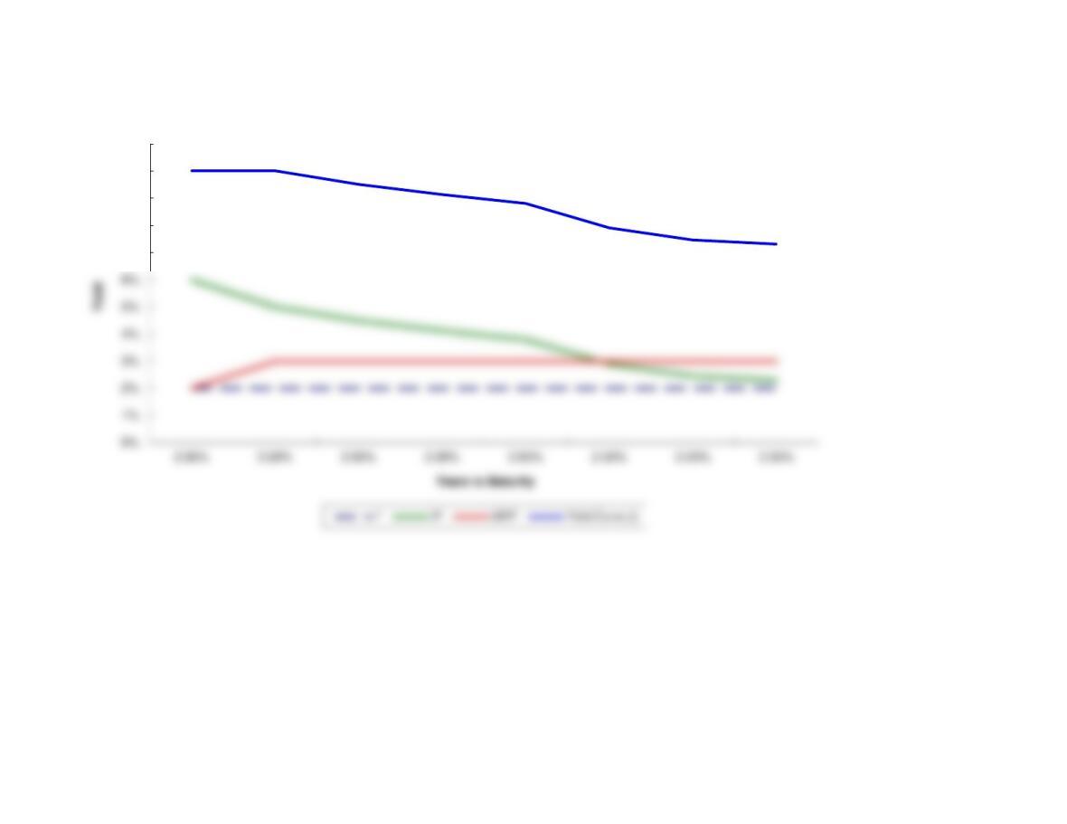
varying maturities. Every security’s yield is based upon investor attitudes and expectations regarding future market
conditions. In other words, the sort of “building” we have done with our yield curves sort of occurs implicitly for
every security.
have little guidance regarding the determination of the default risk premium. However, we could assume that the
relationship between corporate bonds of a given rating and Treasury securities of the same maturity would have a
fairly stable relationship. By that token, we might be able to derive a good point estimator of the default risk premium
by looking at the recent average default spread for different rated corporate bonds. This information is as follows:
22.00% 5.00% 3.00% 10.00% 1.02% 11.02% 2.86% 12.86%
32.00% 4.50% 3.00% 9.50% 1.04% 10.54% 2.91% 12.41%
42.00% 4.13% 3.00% 9.13% 1.06% 10.19% 2.97% 12.10%
52.00% 3.80% 3.00% 8.80% 1.08% 9.88% 3.03% 11.83%
mechanism for simulating this relationship. Just as we did for the maturity risk premium, we will “manufacture” a
relationship by which the default risk premium interacts with the time to maturity. The following formula is simply
made up, but it gives us a default relationship with which we are comfortable.
32
33
34
35
36
37
64
65
66
67
68
69
74
75
76
77
78
79
80
81
90
91
92
93
94
98
99
100
101
102
103
104
105
106
107
108
A B C D E F G H I
Years to Real risk-free Inflation Maturity Risk Treasury
Maturity rate (r*) Premium (IP) Premium (MRP) Yield
12.00% 6.00% 2.00% 10.00%
22.00% 5.00% 3.00% 10.00%
32.00% 4.50% 3.00% 9.50%
30 2.00% 2.30% 3.00% 7.30%
To this point, we have constructed yield curves based upon hypothetical data. The first yield curve operates under
the simple assumption that inflation is expected to rise in the future. To some extent, actual yield curves are
constructed in similar ways. The true Treasury yield curve is determined by graphing Treasury security yields of
CORPORATE BONDS
Default Risk Premiums and the Liquidity Premium
The construction of corporate yields is a process of beginning with the appropriate Treasury yield curve and adding in
these additional yield premiums. However, the determination of these premiums can be tricky. It seems logical that
default risk on corporate bonds should somehow be a function of the firm’s corporate bond rating. Apart from that we
This tells us the average default spreads of corporate securities with various bond ratings. We will use this data as the
starting point for our corporate yield curves. Naturally, the first question that arises is, “Does the default risk premium
change, or does it always stay the same?”. Logically, the idea of a time-varying default risk premium seems fairly
plausible. The longer the maturity of the security, the greater the possibility of default. Therefore, we need some sort of
DRP t = Default spread * (1.02)(t-1)
With all of that having been said, we can step forward and try to construct corporate yield curves.
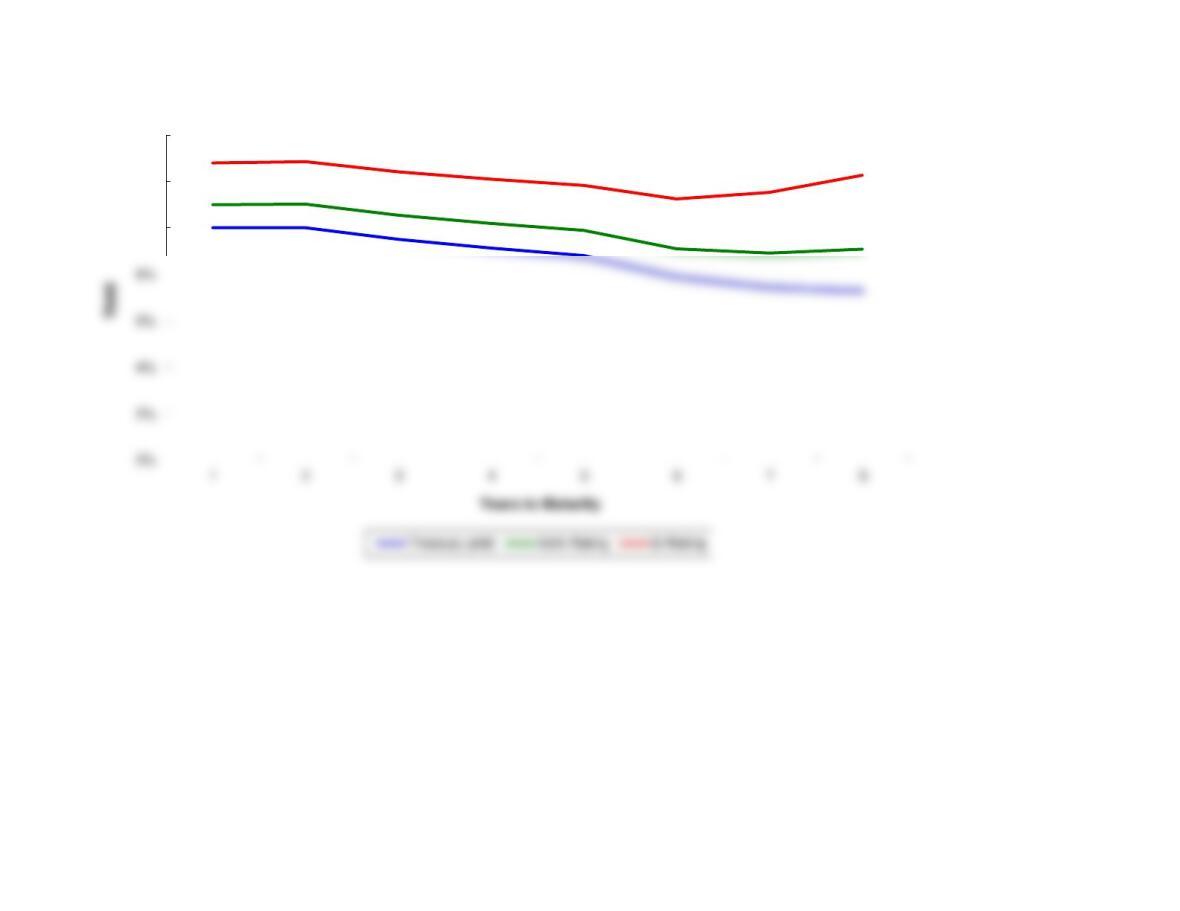
Naturally, yield curves can be created for corporate bonds of any rating. However, we have chosen to create curves for
only AAA and B rated bonds. This exercise is for purely illustrative purposes, so rather than complicate the graph
with a lot of curves, we will create two curves to show the relationship between yield curves.
Years to Real risk-free Inflation Maturity Risk Treasury AAA-rating AAA-rated B-rating B-rated
Maturity rate Premium (IP) Premium (MRP) yield DRP bond yield DRP bond yield
12.00% 6.00% 2.00% 10.00% 1.00% 11.00% 2.80% 12.80%
42.00% 4.13% 3.00% 9.13%
52.00% 3.80% 3.00% 8.80%

117
127
137
138
139
140
A B C D E F G H I
10 2.00% 2.90% 3.00% 7.90% 1.20% 9.10% 3.35% 11.25%
20 2.00% 2.45% 3.00% 7.45% 1.46% 8.91% 4.08% 11.53%
30 2.00% 2.30% 3.00% 7.30% 1.78% 9.08% 4.97% 12.27%
Looking at the yield curve we have constructed, we see a relationship that we should have expected. We see that at any
length to maturity, the yield on corporate bonds is always greater than the yield on Treasuries. This is logical because
corporate securities carry a default risk, and Treasuries do not. Furthermore, we observe that at any length to maturity
the corporate security with the lower rating always has a higher yield than a corporate bond with a higher rating. Once
again, this is a logical conclusion. Remember, a bond rating, among other things, gives you an indication of the
expected possibility of default. Naturally, this possibility is greater for bonds with lower ratings, and this possibility of
default gives the indicated security greater risk. Greater risk should result in a higher yield.
7%
8%
9%
10%
11%
10%
12%
14%

We have already entered the base case data for each model in this
file, and the models have performed the analysis for preceding parts
of the problem. You will need to enter the data for each of the
remaining parts of the problem–we indicate in each problem the parts
that should be done using the spreadsheet. However, there are several
points worth noting before you go into a model:
1. The input data are entered in specified cells in the INPUT DATA
section. When you change an input item, the model automatically
2. The key output data are displayed to the right of the INPUT DATA
section or immediately below it. This placement permits you to
change an input and instantly see how that change affects the output
of the model. This is extremely useful in sensitivity analysis.
3. Input data items that you can change are distinguished from the
ones you should not change. The items that you can change are
highlighted in color (blue) whereas the other items are printed in black.
4. All percentages must be entered as decimals. Dollars and other
numbers must be entered without dollar signs or commas.
5. Instructions and comments concerning specific models accompany
each model. Graphs associated with the model are included in
another worksheet that can be accessed by clicking on the
worksheet labeled GRAPH at the bottom of the spreadsheet.
GENERAL INSTRUCTIONS FOR COMPUTERIZED PROBLEM SOLUTIONS
recalculates the values of appropriate output data items, unless
you are told otherwise. If the values do not change automatically,