CFIN6 – CHAPTER 4
INTEGRATIVE PROBLEM SOLUTION
a. Discuss basic time value concepts, terminology, and solution methods. A cash flow timeline is a graphical
representation that is used to show the timing of cash flows. The tick marks represent end of periods (often
years), so time 0 is today; time 1 is the end of the first year, or 1 year from today; and so on.
LUMP-SUM AMOUNT—a single flow; for example, a $100 inflow in Year 2:
0 1 2 3 Year
100 Cash flow
UNEVEN CASH FLOW STREAM—an irregular series of cash flows that do not constitute an annuity:
0 1 2 3 Year
–50 100 75 –50 Cash flow
After 1 year:
FV1 = PV + INT1 = PV + PV(r) = PV(1 + r) = $100(1.10) = $110.00.
Similarly:
FV2 = FV1 + INT2 = FV1 + FV1(r)
r%
r%

In general, we see that:
FVn = PV(1 + r)n,
so FV3 = $100(1.10)3 = $100(1.3310) = $133.10.
(1) Numerical approach—use a regular calculator: FV3 = $100(1.10)3 = $133.10.
(2) Financial calculator: This is especially efficient for more complex problems, including exam problems.
Input the following values: N = 3, I/Y = 10, PV = –100, and PMT = 0; compute FV = $133.10.
Step 1: Set up the spreadsheet:
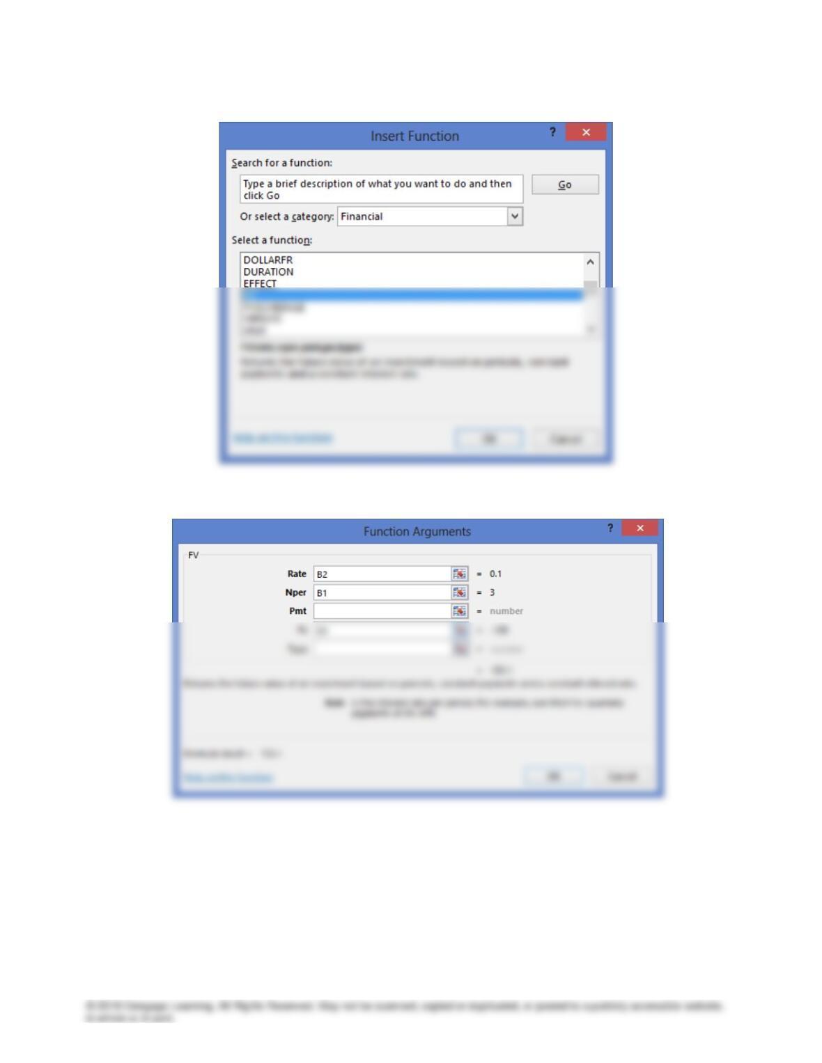
Step 2: Select FV in the financial function category:
Step 3: Input the cell locations of the data:
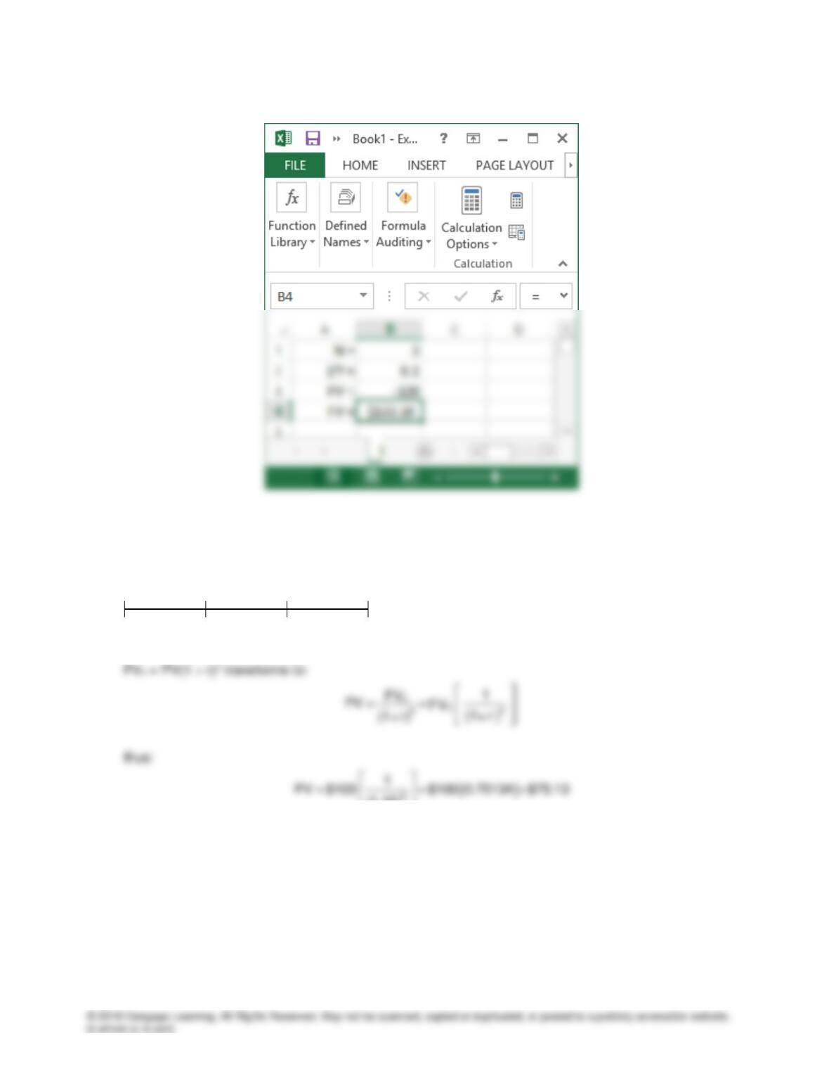
Step 4: Press OK to display the solution:
b(2). Finding present values, or discounting (moving to the left along the timeline), is the reverse of
compounding, and the basic present value equation is the reciprocal of the compounding equation:
0 1 2 3
PV = ? 100
(1.10)
The same methods (regular calculator, financial calculator, and spreadsheet) used for finding future values
also are used to find present values, which is called discounting.
Numerical (regular calculator) solution: Given above.
Financial calculator solution: Input N = 3, I/Y = 10, PMT = 0, and FV = 100; compute PV = $75.13.
Spreadsheet solution: Use the PV financial function that is available on the spreadsheet.
10%
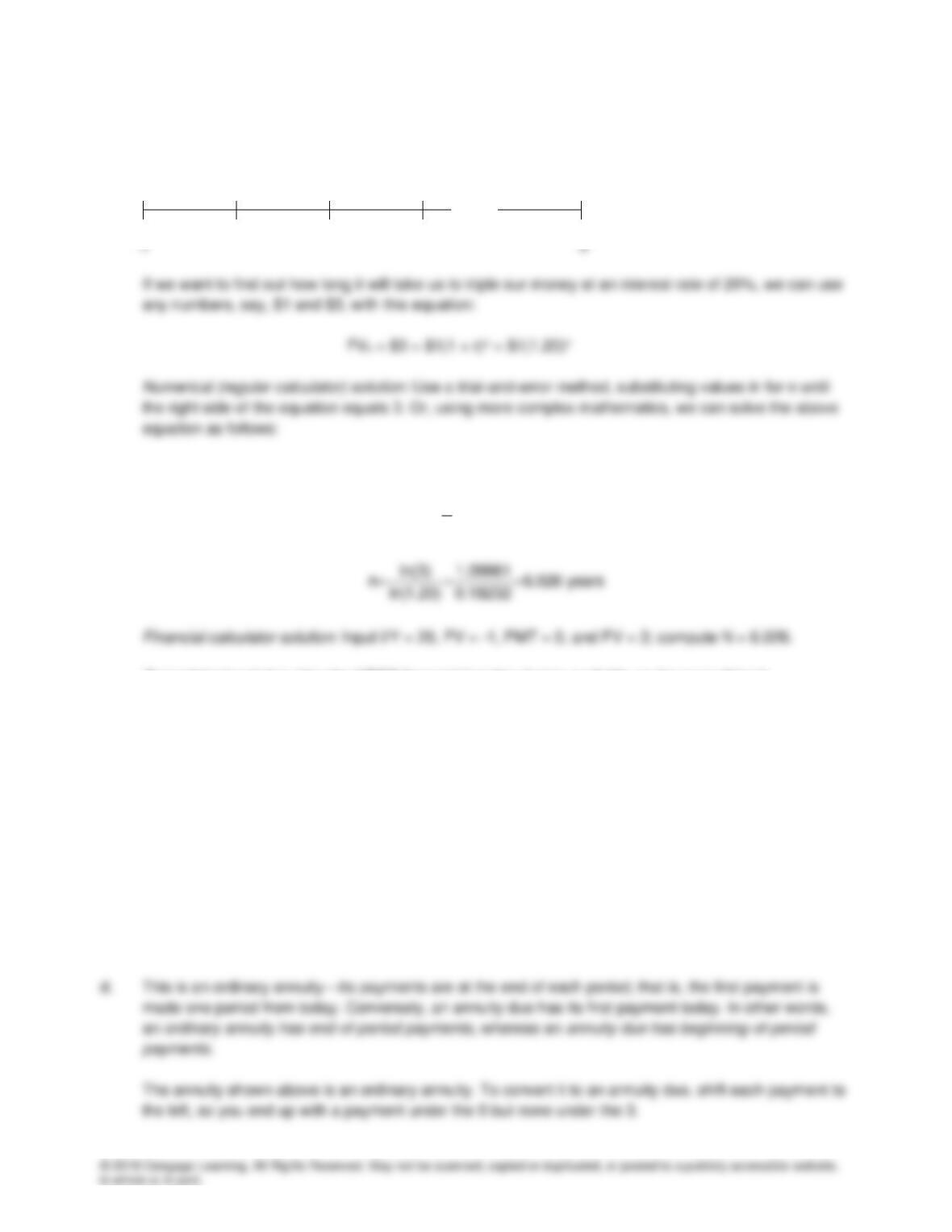
c. We have this situation in timeline format:
0 1 2 3 n = ?
n
n
3 1(1.20)
3
(1.20) 1
=
=
Spreadsheet solution: Use the NPER financial function that is available on the spreadsheet.
Thus, it takes approximately 6 periods for an amount to triple at a 20% interest rate.
***************************************************************************************
OPTIONAL QUESTION: A FARMER CAN SPEND $60 PER ACRE TO PLANT PINE TREES ON SOME
MARGINAL LAND. THE EXPECTED REAL RATE OF RETURN IS 4%, AND THE EXPECTED
INFLATION RATE IS 6%. WHAT IS THE EXPECTED VALUE OF THE TIMBER AFTER 20 YEARS?
FV20 = $60(1 + 0.04 + 0.06)20 = $60(1.10)20 = $403.65 per acre.
We could have asked: How long would it take $60 to grow to $403.65, given the real rate of return of 4%
and an inflation rate of 6%. Of course, the answer would be 20 years.
***************************************************************************************
20%
…
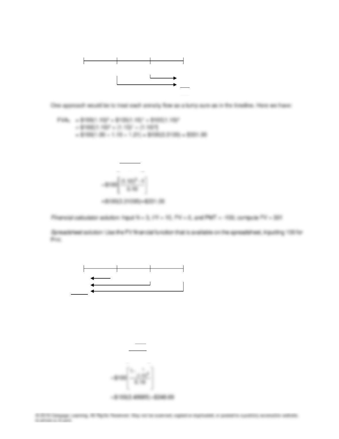
e(1). 0 1 2 3
100 100 100
110
121
331
Numerical solution:
n
n
(1 r) 1
FVA PMT r
+−
=
e(2). 0 1 2 3
90.91 100 100 100
82.64
75.13
248.68
The present value of the annuity is $248.68. Here we used the lump sum approach, but the same result
could be obtained by using a regular or financial calculator.
Numerical solution:
1n
(1 r)
n
1
PVA PMT r
+
−
=
10%
10%
Financial calculator solution: Input N = 3, I/Y = 10, PMT = 100, and FV = 0; compute PV = -248.69
Spreadsheet solution: Use the PV financial function that is available on the spreadsheet, inputting 100 for
PMT.
e(3). If the annuity were an annuity due, each payment would be shifted to the left, so each payment is
compounded over an additional period or discounted back over one less period.
Future Value of the Annuity:
Numerical solution:
0.10
$100(3.64100) $364.10
==
Financial calculator solution: Switch your calculator to “BEG” or beginning or “DUE” mode, input N = 3, I/Y
= 10, PV = 0, and PMT = –100; compute FV = 364.10. Remember to change back to “END” mode after
working an annuity due problem with your calculator.
Numerical solution:
1n
(1 r)
n
1
PVA(DUE) PMT (1 r)
r
+
−
= +
Spreadsheet solution: Use the PV financial function that is available on the spreadsheet, inputting PMT
= 100 and Type =1.
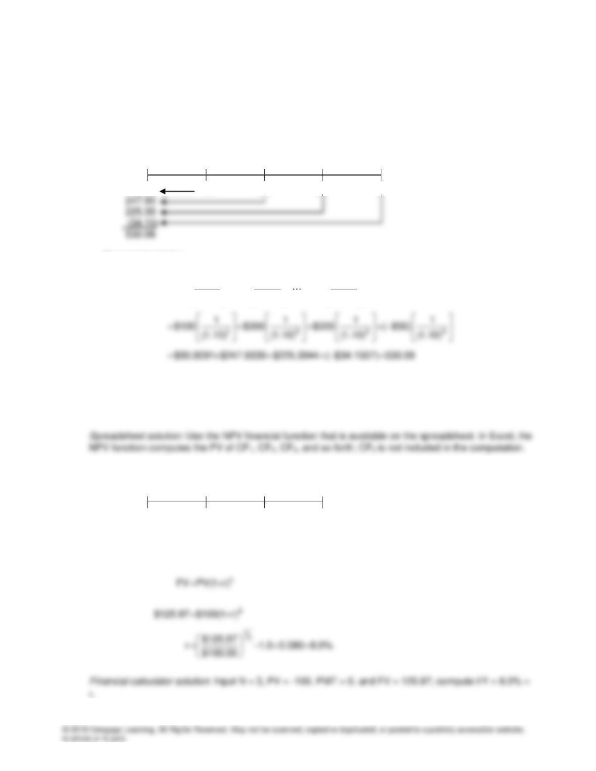
f. Here we have an uneven cash flow stream. The most straightforward approach is to find the present
value of each cash flow and then sum the PVs as shown below:
0 1 2 3 4
90.91 100 300 300 –50
Numerical solution:
1 2 n
1 2 n
1 1 1
PV CF CF CF
(1 r) (1 r) (1 r)
= + + +
+ + +
Financial calculator solution: Financial calculators have cash flow (CF) functions in which you would
input the cash flows, so they are in the calculator’s memory, input the interest rate, I, and then compute
the NPV, which is the present value. In this case, CF0 = 0, CF1 = 100, CF2 = 300, CF3 = 300, and CF4
= –50.
g. 0 1 2 3
–100 125.97
FV = $100(1 + r)3 = $125.97
Numerical solution:
10%
r = ?
Spreadsheet solution: Use the RATE financial function that is available on the spreadsheet
h(1). Investments that pay interest more frequently than once per year, for example—semiannually, quarterly, or
h(2). The quoted, or simple, rate is merely the quoted percentage rate of return, the periodic rate is the rate
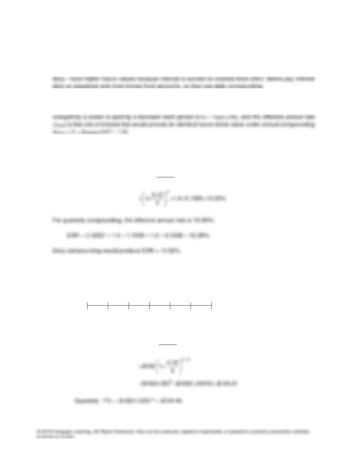
h(3). The effective annual rate for 10% semiannual compounding, is 10.25%:
m
SIMPLE
r
EAR = 1 + – 1.0
m
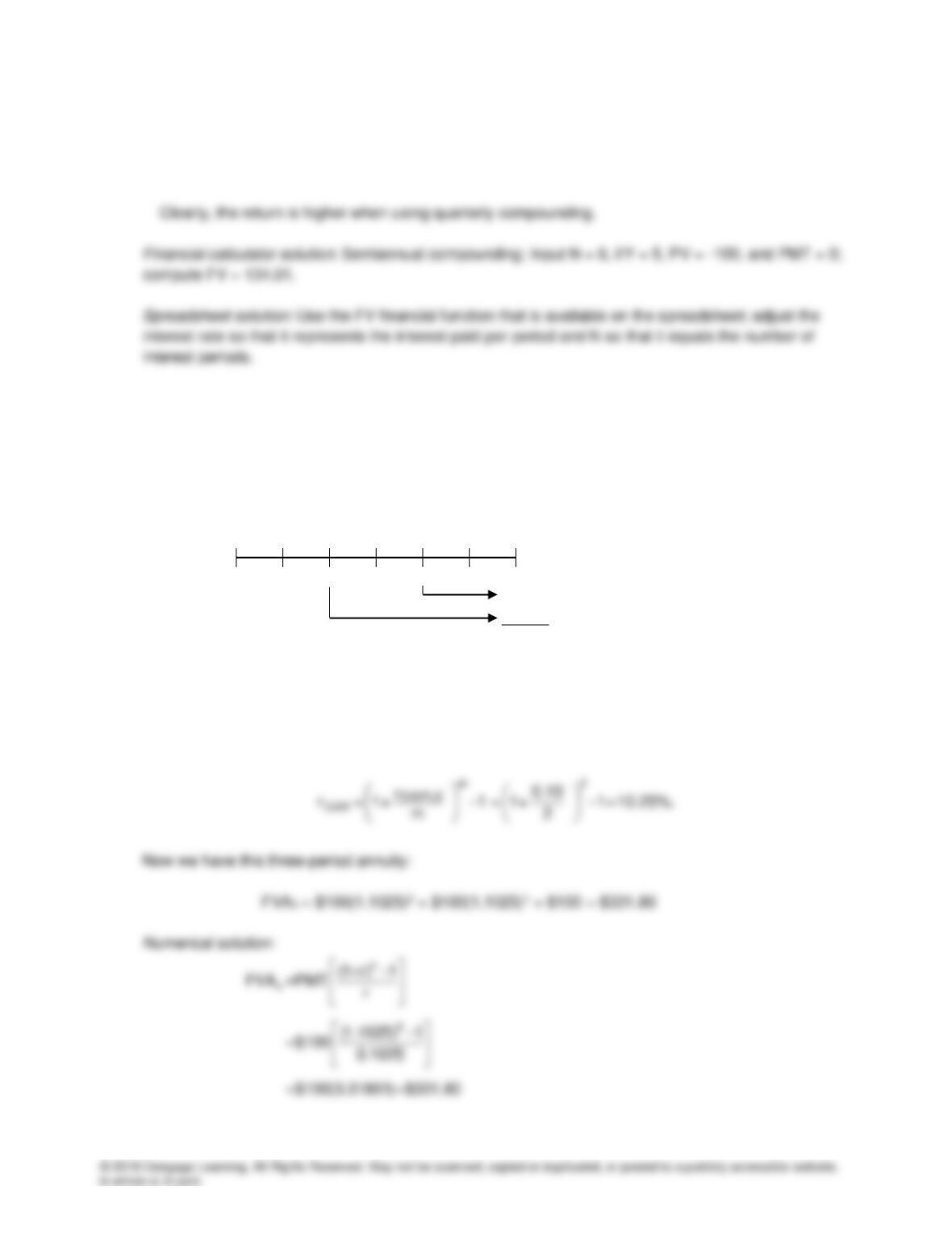
h(4). With semiannual compounding, the $100 is compounded over six semiannual periods at a 5.0% periodic
rate:
1 2 3 Years
0 1 2 3 4 5 6 Six-month periods
–100 FV=?
Numerical Solution:
mn
SIMPLE
n
r
FV PV 1
m
=+
5%
Another approach here would be to use the effective annual rate and compound over annual periods:
Semiannually: $100(1.1025)3 = $134.01
Quarterly: $100(1.1038)3 = $134.49
i. If annual compounding is used, then the simple rate will be equal to the effective annual rate. If more
frequent compounding is used, the effective annual rate will be greater than the simple rate. That is, rSIMPLE
= rPER = rEAR when interest is compounded annually, whereas rSIMPLE < rEAR when interest is compounded
more than once per year.
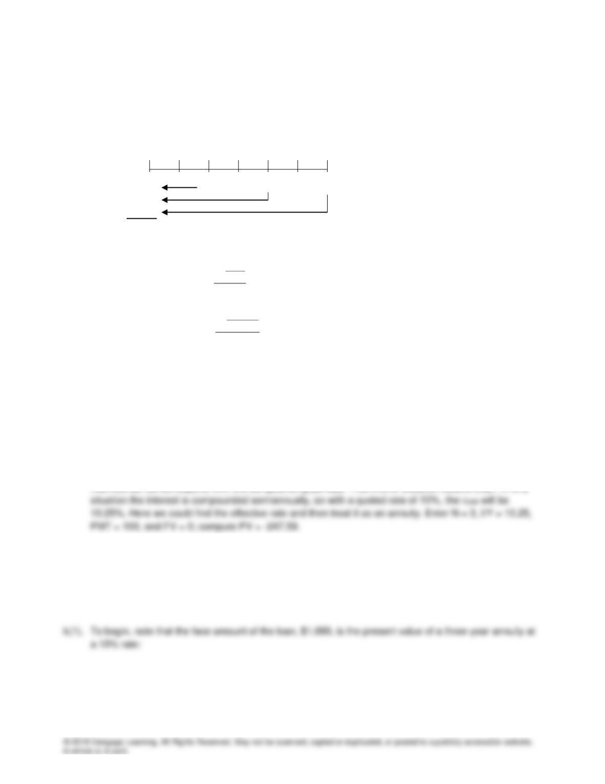
j(1). 0 1 2 3
100 100 100.00
110.25 = $100(1.05)2
121.55 = $100(1.05)4
331.80
Here we have a different situation. The payments occur annually, but compounding occurs each six
months. Thus, we cannot use normal annuity valuation techniques. There are two approaches that can
be applied: (1) Treat the cash flows as lump sums, as was done above, or (2) Treat the cash flows as
an ordinary annuity, but use the effective annual rate:
5%
Financial calculator solution: Input N = 3, I/Y = 10.25, PV = 0, and PMT = -100; compute FV = 331.80
Spreadsheet solution: Use the FV financial function that is available on the spreadsheet, inputting 100 for
Pmt and 0.1025 for Rate.
j(2). 0 1 2 3
90.70 100 100 100
82.27
74.62
247.59
Numerical solution:
1n
(1 r)
n
13
(1.1025)
1
PVA PMT r
1
$100 0.1025
$100(2.47595) $247.59
+
−
=
−
=
==
Financial calculator solution: Input N = 3, I/Y = 10.25, PMT = 100, and FV = 0; compute PV = -247.59
Spreadsheet solution: Use the PV financial function that is available on the spreadsheet, inputting 100 for
Pmt and 0.1025 for Rate.
j(3). The payment stream is an annuity in the sense of constant amounts at regular intervals, but the
j(4). rSIMPLE can only be used in the calculations when annual compounding occurs. If the simple rate of
10% was used to discount the payment stream the present value would be overstated by $272.32 –
$247.59 = $24.73.
5%
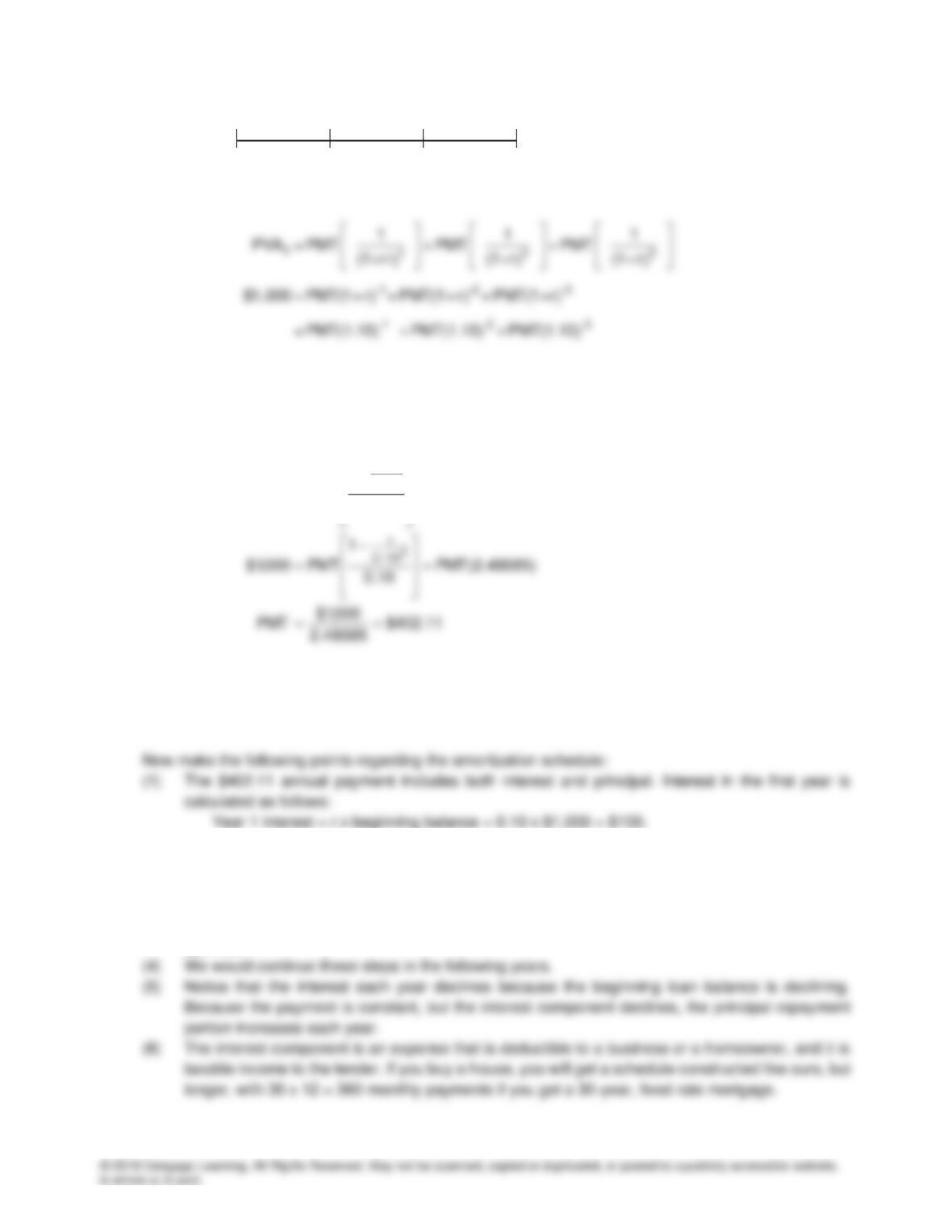
0 1 2 3
–1,000 PMT PMT PMT
We have an equation with only one unknown, so we can solve it to find PMT.
Numerical solution:
r
1
PMTPVA
n
)r1(
1
n
−
=+
Financial calculator solution: Input N = 3, I/Y = 10, PV = 1,000, and FV = 0; compute PMT = –402.11
Spreadsheet solution: Use the PV financial function that is available on the spreadsheet, solving for Pmt.
(2) The repayment of principal is the difference between the $402.11 annual payment and the interest
payment:
Year principal repayment = $402.11 – $100 = $302.11.
(3) The loan balance at the end of the first year is:
Year 1 ending balance = beginning balance – principal repayment = $1,000 – $302.11 =
$697.89.
10%
(7) The payment might have to be increased by a few cents in the final year to take care of rounding
errors and make the final payment produce a zero ending balance.
The amortization schedule would be:
Beginning Interest Principal Ending
Year Balance Payment @ 10% Repayment Balance
1 $1,000.00 $402.11 $100.00 $302.11 $697.89
2 697.89 402.11 69.79 332.32 365.57
3 365.57 402.11 36.56 365.55 0.02 (rounding difference)
l. First, determine the effective annual rate of interest, with daily compounding:
365
0.1133463
EAR = 1 + 1 = 0.12 = 12.0%.
365
−
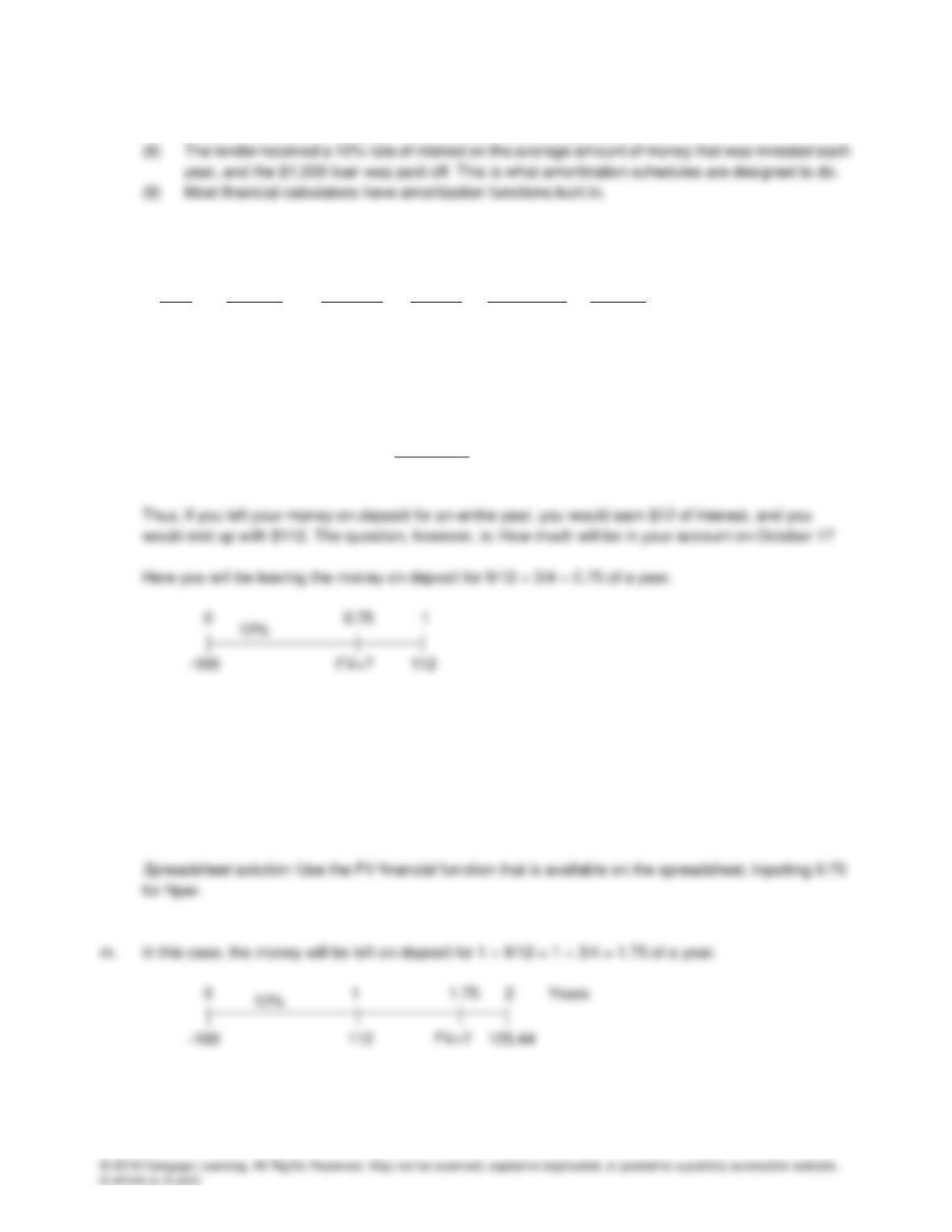
You would use the regular set-up, but with the fraction of the year:
Numerical solution:
FV0.75 = $100(1.12)0.75 = $100(1.08871) = $108.87
Financial calculator solution: Input N = 0.75, I/Y = 12, PV = -100, and PMT = 0; compute FV = 108.87
Numerical solution:
FV1.75 = $100(1.12)1.75 = $100(1.21936) = $121.94
Financial calculator solution: Input N = 1.75, I/Y = 12, PV = -100, and PMT = 0; compute FV = 121.94
Spreadsheet solution: Use the FV financial function that is available on the spreadsheet, inputting 1.75
for Nper.
(1) Future Value
Numerical solution:
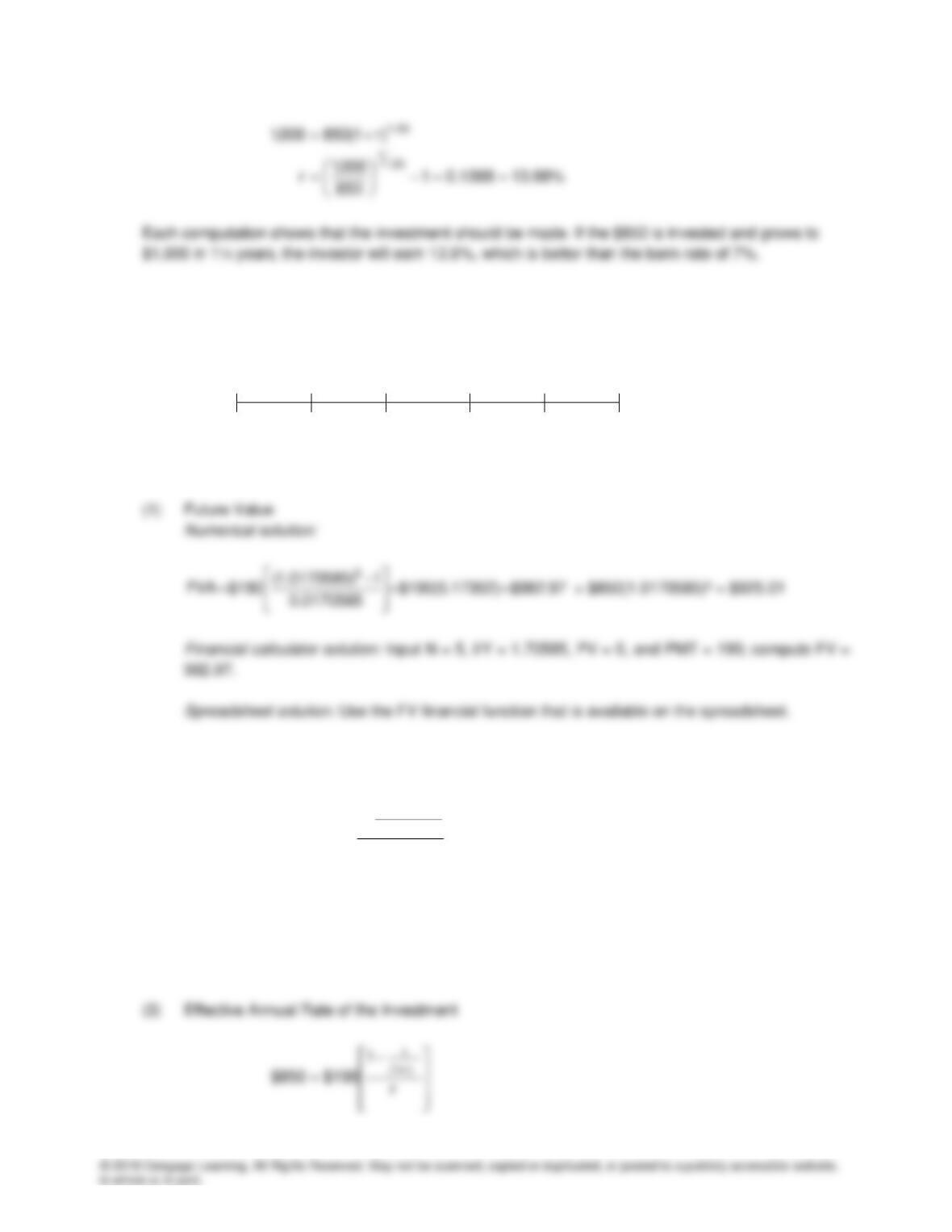
FV1.25 = $850(1.07)1.25 = $850(1.08825) = $925.01 < $1,000 FV of investment
1.25
1
PV $1,000 $1,000(0.91890) $918.90
(1.07)
= = =
> $850 cost of investment
Financial calculator solution: Input N = 1.25, I/Y = 7, PMT = 0, and FV = 1,000; compute PV = –
918.90
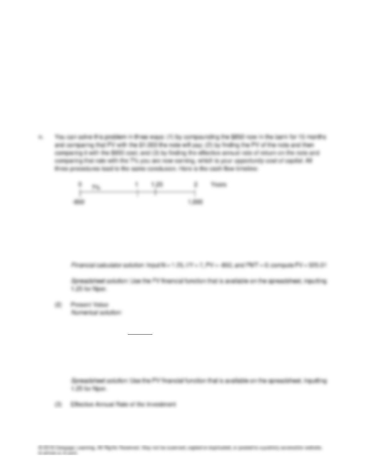
o. Here is the cash flow timeline:
¼ ½ ¾ 1 1¼ Years
0 1 2 3 4 5 Quarters
850 190 190 190 190 190
Rate per period = (1.07)0.25 – 1.0 = 1.70585
(2) Present Value
Numerical solution:
1
(1.0170585)
1
PVA $190 $190(4.75397) 903.25
0.0170585
−
= = =
Financial calculator solution: Input N = 5, I/Y = 1.70585, PMT = 190, and FV = 0; compute PV = –
903.25
Spreadsheet solution: Use the PV financial function that is available on the spreadsheet.
1.706%

Numerical solution: Use a trial-and-error method to determine r.
Financial calculator solution: Input N = 5, PV = –850, PMT = 190, and FV = 0; compute I/Y = 3.8259
per quarter. EAR = (1.038259)4 – 1 = 0.1620 = 16.20% > 7% on bank deposit.
Each computation shows that the investment should be made.