IFM12 Ch03 Mini Case prd.xlsx Mini Case
1/6/2015
Answer the following questions.
Expected return of a portfolio:
Standard deviation of a portfolio:
Asset A Asset B
Expected return, r hat 10% 16%
Standard deviation, s20% 40%
Correlation = 0.35
Proportion of Portfolio in
Security A
(Value of wA)
Proportion of
Portfolio in
Security B
(Value of 1-wA)
rpsp
1.00 0.00 10.00% 20.00%
0.90 0.10 10.60% 19.76%
Chapter 3. Mini Case
a. Suppose Asset A has an expected return of 10 percent and a standard deviation of 20 percent. Asset
B has an expected return of 16 percent and a standard deviation of 40 percent. If the correlation between
A and B is 0.35, what are the expected return and standard deviation for a portfolio comprised of 30
percent Asset A and 70 percent Asset B?
b. Plot the attainable portfolios for a correlation of 0.35. Now plot the attainable portfolios for
correlations of +1.0 and -1.0.
portfolio with different percentages invested in each asset.
rAB = +0.35: Attainable Set of Risk/Return
0.80 0.20 11.20% 20.24%
0.70 0.30 11.80% 21.39%
0.60 0.40 12.40% 23.12%
0.50 0.50 13.00% 25.30%
0.40 0.60 13.60% 27.83%
0.30 0.70 14.20% 30.62%
0.20 0.80 14.80% 33.61%
0.00 1.00 16.00% 40.00%
IFM12 Ch03 Mini Case prd.xlsx Mini Case
Correlation = 1
Proportion of Portfolio in
Security A
(Value of wA)
Proportion of
Portfolio in
Security B
(Value of 1-wA)
rpsp
1.00 0.00 10.00% 20.00%
0.90 0.10 10.60% 21.59%
Correlation = -1
Proportion of Portfolio in
Security A
(Value of wA)
Proportion of
Portfolio in
Security B
(Value of 1-wA)
rpsp
1.00 0.00 10.00% 20.00%
0.90 0.10 10.60% 14.63%
0.80 0.20 11.20% 9.80%
0.70 0.30 11.80% 6.78%
0.60 0.40 12.40% 8.00%
0.50 0.50 13.00% 12.25%
0.40 0.60 13.60% 17.44%
0.30 0.70 14.20% 22.93%
0.20 0.80 14.80% 28.57%
0.10 0.90 15.40% 34.26%
0.00 1.00 16.00% 40.00%
5%
10%
Expected return
15%
20%
rAB = +1.0: Attainable Set of Risk/Return
Combinations
10%
20%
Expected return
rAB = -1.0: Attainable Set of Risk/Return
Combinations
Michael C. Ehrhardt Page 2 3/1/2023
0.80 0.20 11.20% 23.32%
0.70 0.30 11.80% 25.18%
0.60 0.40 12.40% 27.13%
0.50 0.50 13.00% 29.15%
0.40 0.60 13.60% 31.24%
0.30 0.70 14.20% 33.38%
0.20 0.80 14.80% 35.55%
0.10 0.90 15.40% 37.76%
0.00 1.00 16.00% 40.00%
IFM12 Ch03 Mini Case prd.xlsx Mini Case
Asset A Risk-free Asset
Expected return, r hat 10% 5%
Standard deviation, s20% 0%
Proportion of Portfolio in
Security A
(Value of wA)
Proportion of
Portfolio in
Risk-free Asset
(Value of 1-wA)
rpsp
1.00 0.00 10.00% 20.00%
0.90 0.10 9.50% 18.00%
0.80 0.20 9.00% 16.00%
0.70 0.30 8.50% 14.00%
0.60 0.40 8.00% 12.00%
0.50 0.50 7.50% 10.00%
FEASIBLE AND EFFICIENT PORTFOLIOS
The feasible set of portfolios represent all portfolios that can be constructed from a given set of stocks.
An efficient portfolio is one that offers: the most return for a given amount of risk or the least risk for a
given amount of return.
c. Suppose a risk-free asset has an expected return of 5 percent. By definition, its standard deviation is
zero, and its correlation with any other asset is also zero. Using only Asset A and the risk-free asset, plot
the attainable portfolios.
d. Construct a reasonable, but hypothetical, graph that shows risk, as measured by portfolio standard
deviation, on the X axis and expected rate of return on the Y axis. Now add an illustrative feasible (or
attainable) set of portfolios, and show what portion of the feasible set is efficient. What makes a
particular portfolio efficient? Don’t worry about specific values when constructing the graph-merely
illustrate how things look with “reasonable” data.
10%
10%
15%
Attainable Set of Risk/Return Combinations
with Risk-Free Asset
Michael C. Ehrhardt Page 3 3/1/2023
portfolio with different percentages invested in each asset.
IFM12 Ch03 Mini Case prd.xlsx Mini Case
OPTIMAL PORTFOLIOS
An investor’s optimal portfolio is defined by the tangency point between the efficient set and the investor’s
indifference curve. The indifference curve reflect an investor’s attitude toward risk as reflected in his or
her risk/return trade off function.
f. What is the Capital Asset Pricing Model (CAPM)? What are the assumptions that underlie the model?
CAPM
The Capital Asset Pricing Model is an equilibrium model that specifies the relationship between risk and
required rate of return for assets held in well diversified portfolios.
Assumptions
Investors all think in terms of a single holding period.
e. Now add a set of indifference curves to the graph created for part b. What do these curves represent?
What is the optimal portfolio for this investor? Finally, add a second set of indifference curves which
leads to the selection of a different optimal portfolio. Why do the two investors choose different
portfolios?
Expected
Portfolio
Return, r p
Efficient Set
Feasible Set
IB2IB1
Expected
Return, r p
Michael C. Ehrhardt Page 4 3/1/2023
All investors have identical expectations.
Investors can borrow or lend unlimited amounts at the risk free rate.
All assets are perfectly divisible.
There are not taxes and transaction costs.
Quantities of all assets are given and fixed.
g. Now add the risk-free asset. What impact does this have on the efficient frontier?
IFM12 Ch03 Mini Case prd.xlsx Mini Case
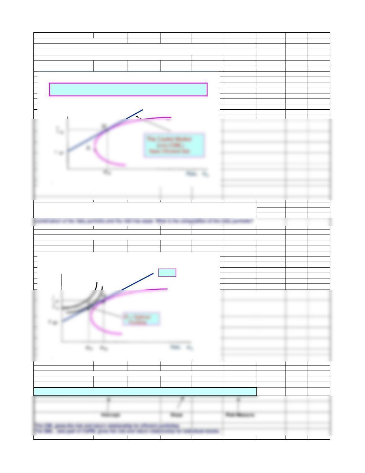
EFFICIENT SET WITH A RISK-FREE ASSET
When a risk free asset is added to the feasible set, investors can create portfolios that combine this asset
with a portfolio of risky asset. The straight line connecting rrf with M, the tangency point between the line
and the old efficiency set, becomes the new efficient frontier.
OPTIMAL PORTFOLIO WITH A RISK-FREE ASSET
The optimal portfolio for any investor is the point of tangency between the CML and the investors indifference
curve.
Capital Market Line
The capital market line is all linear combinations of the risk free asset and portfolio M.
rhat= rrf + (rm-rrf)/smxsp
combination of the risky portfolio and the risk-free asset. What is the composition of the risky portfolio?
h. Write out the equation for the Capital Market Line (CML) and draw it on the graph. Interpret the CML.
Now add a set of indifference curves, and illustrate how an investor’s optimal portfolio is some
Z
Efficient Set with a Risk-Free Asset
Expected
Return, r p
I1
I2
CML
Expected
Return, r p
Michael C. Ehrhardt Page 5 3/1/2023
The CML gives the risk and return relationship for efficient portfolios
The SML , also part of CAPM, gives the risk and return relationship for individual stocks.
IFM12 Ch03 Mini Case prd.xlsx Mini Case
SML =
ri + (RPm) x b
Beta Calculation
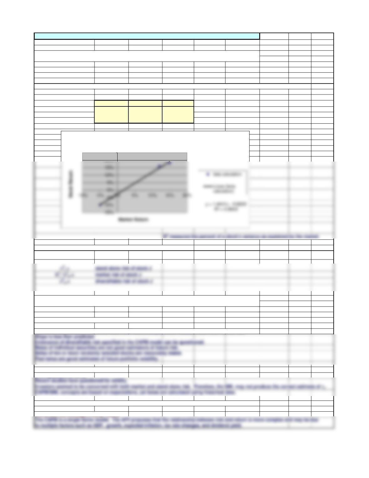
Run a regression line of past returns on Stock I versus returns on the market. The regression line is the characteristic line.
Year
rMri
115% 18%
2-5% -10%
312% 16%
Relationship between stand alone, market, and diversifiable risk
s2j = b2j *s2m + s2ej
Test to verify CAPM
Beta stability test and tests based on the slope of the SML.
Test of the SML indicate a more-or-less linear relationship between realized return and market risk.
Slope is less than predicted
Irrelevance of diversifiable risk specified in the CAPM model can be questioned.
Betas of individual securities are not good estimators of future risk.
Betas of ten or more randomly selected stocks are reasonably stable.
Past betas are good estimates of future portfolio volatility.
Conclusions regarding CAPM
It is impossible to verify.
Recent studies have questioned its validity.
Investors seemed to be concerned with both market and stand alone risk. Therefore, the SML may not produce the correct estimate of rj.
CAPM/SML concepts are based on expectations, yet betas are calculated using historical data.
k. Briefly explain the difference between the CAPM and the Arbitrage Pricing Theory (APT).
CAPM and the Arbitrage Pricing Theory
The CAPM is a single factor model. The APT proposes that the relationship between risk and return is more complex and may be due
to multiple factors such as GDP, growth, expected inflation, tax rate changes, and dividend yield.
j. What are two potential tests that can be conducted to verify the CAPM? What are the results of such
tests? What is Roll’s critique of CAPM tests?
i. What is a characteristic line? How is this line used to estimate a stock’s beta coefficient? Write out and
explain the formula that relates total risk, market risk, and diversifiable risk.
25%
Beta Calculation
Michael C. Ehrhardt Page 6 3/1/2023