Finance Chapter 3 Investors can borrow or lend unlimited amounts

Answers and Solutions: 3 – 1

Chapter 3

Risk and Return: Part II

ANSWERS TO BEGINNING-OF-CHAPTER QUESTIONS

We do not normally cover the material in Chapter 3 in depth in our intermediate financial

management course—this treatment is reserved for the investments course—but it is useful

for students to recognize that the CAPM results were derived under some restrictive

assumptions and hence the derived equations do not necessarily describe how returns are

established in the real world.

3-1 In finance theory, the value of an investment is found as the PV of the asset’s expected

stream of cash flows. The CAPM is an “asset pricing theory” that specifies how the

discount rate in the valuation equation should be determined. Although the theory is

quite complex and has many component parts, its “bottom line” is the SML equation,

often called the CAPM equation:

developed the SML as shown back in Figure 2-10 and Equation 2-9.

A number of simplifying assumptions, including the following, were made in order to

derive the CAPM:

1. Investors focus on a single holding period.

2. Investors can borrow or lend unlimited amounts at the riskless rate.

3-2 Covariance shows how two variables move in relation to one another. There are different

“states of nature,” each with a probability of occurrence, and a return on each asset under

each state. This probability data can be used to determine the SD of returns for each

asset, the variance of those returns, and the correlation between returns on the different

assets.

3-3 An efficient portfolio is one that produces the highest expected return for any given level

of risk. Markowitz showed how to find the frontier of risk and returns for stocks; see

Figure 3-3. Only portfolios on the frontier are efficient. Sharpe added the riskless asset

return and noted that returns on a line connecting rrf and the tangency point on the

efficient frontier was also “feasible” in the sense that portfolios consisting of some of the

Answers and Solutions: 3 – 3

3-4 The SML is essentially derived from the CML. Note that the slope of the CML shows

how much additional return is required for assuming the risk of the market portfolio, i.e.,

the market risk premium (RPM). By definition, the average stock has a beta of 1.0.

3-5 An historical beta is simply the slope of a regression line between returns on a stock and

returns on some market index during some past period. Historical betas can vary

significantly depending on the length of the holding period used (i.e., days, weeks,

months, or years) and the number of time periods included (i.e., the number of years of

data used). There is no “theoretically correct” procedure, and what’s “theoretically

correct” probably varies from investor to investor and over time for a given investor. For

The concept of fundamental betas was developed by Barr Rosenberg, a professor at

Cal-Berkeley, to take account of the fact that fundamental conditions within companies

change over time, and those changes might not be reflected in historical betas. For

example, it is well recognized that the more financial leverage a company uses, the higher

its beta should be. However, if the historical beta is calculated using say 5 years of

monthly data, and if the company changes its capital structure toward the end of the 5

year period, then the historical beta may not reflect the risk for the company in the future,

which is what we are really interested in. Other fundamental factors such as the type of

assets the company is investing in, or conditions in its industry (such as the electric

3-6 As noted above and in the text, the CAPM has not been empirically verified. The biggest

problem, in our minds, is that the theory is based on expectations, yet the tests generally

3-7 A diversifiable risk is a risk that can be eliminated by diversification, while a non-

diversifiable risk is one that cannot be diversified away. Market risk is the non-

diversifiable risk of most concern in financial analysis.

3-8 Undiversified investors bear more risk than diversified investors, and thus they might

argue that they should receive a higher return to compensate for this risk. However, this

is not possible for traded securities, because a given security can have but one price at

Answers and Solutions: 3 – 6

ANSWERS TO END-OF-CHAPTER QUESTIONS

3-1 a. A portfolio is made up of a group of individual assets held in combination. An asset

that would be relatively risky if held in isolation may have little, or even no risk if

held in a well-diversified portfolio.

b. An indifference curve is the risk/return trade-off function for a particular investor and

reflects that investor’s attitude toward risk. The indifference curve specifies an

investor’s required rate of return for a given level of risk. The greater the slope of the

indifference curve, the greater is the investor’s risk aversion.

c. The Capital Asset Pricing Model (CAPM) is a general equilibrium market model

developed to analyze the relationship between risk and required rates of return on

assets when they are held in well-diversified portfolios. The SML is part of the

CAPM.

d. The characteristic line for a particular stock is obtained by regressing the historical

returns on that stock against the historical returns on the general stock market. The

e. Arbitrage Pricing Theory (APT) is an approach to measuring the equilibrium

risk/return relationship for a given stock as a function of multiple factors, rather than

3-2 Security A is less risky if held in a diversified portfolio because of its lower beta and

negative correlation with other stocks. In a single-asset portfolio, Security A would be

Answers and Solutions: 3 – 8

SOLUTIONS TO END-OF-CHAPTER PROBLEMS

3-1 bi = iM (i / M) = 0.70(0.40/0.20) = 1.4.

3-4 a. .)rr(rb)rr(rr

M

iiM

RFMRFiRFMRFi 







With some arranging, the similarities between the CML and SML are obvious. When

in this form, both have the same market price of risk, or slope, (rM – rRF)/σM.

The measure of risk in the CML is σp. Since the CML applies only to efficient

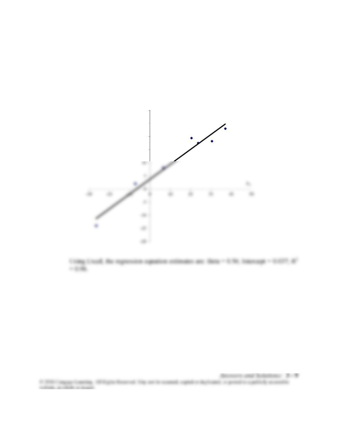
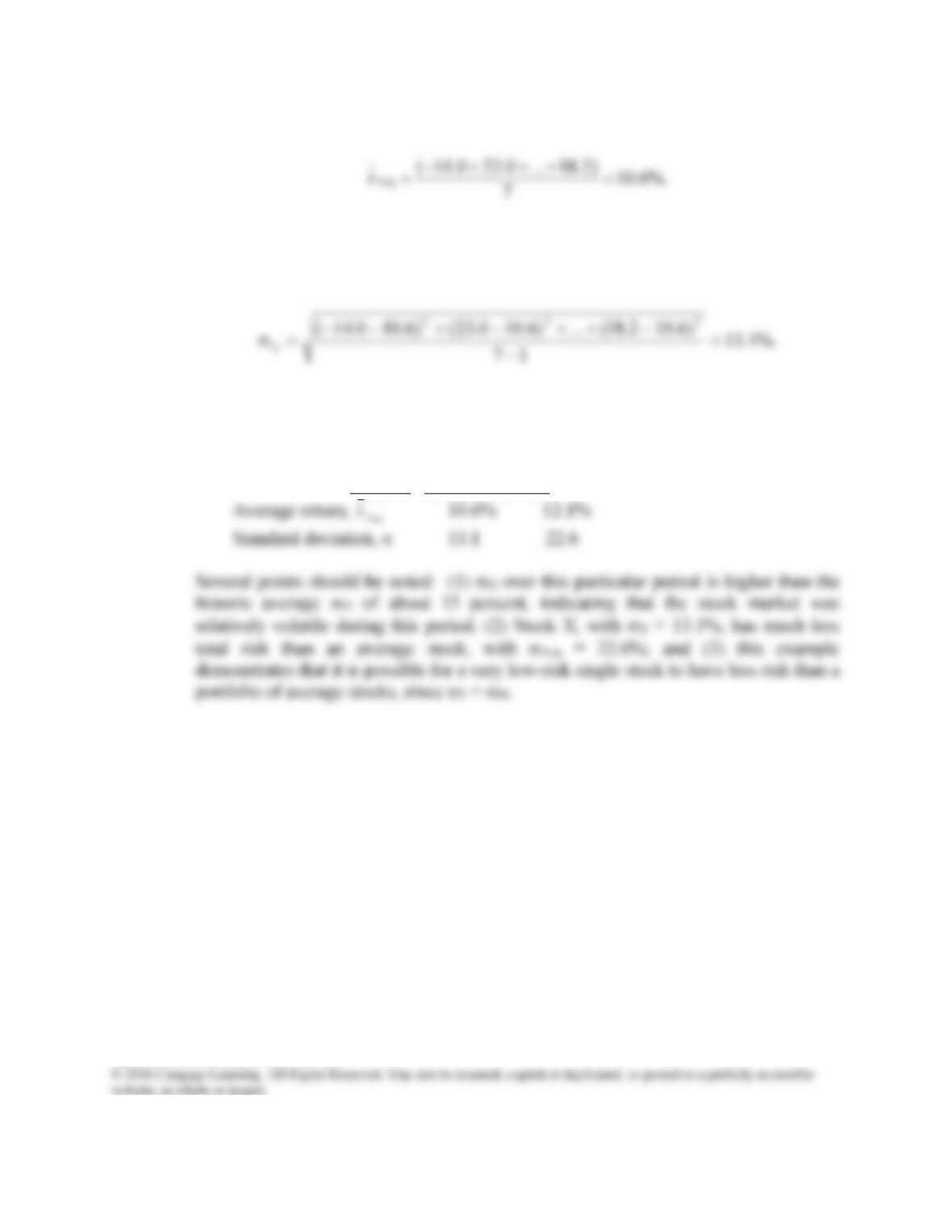
3-5 a. A plot of the approximate regression line is shown in the following figure:

15

20

25

30

rX(%)

Answers and Solutions: 3 – 10

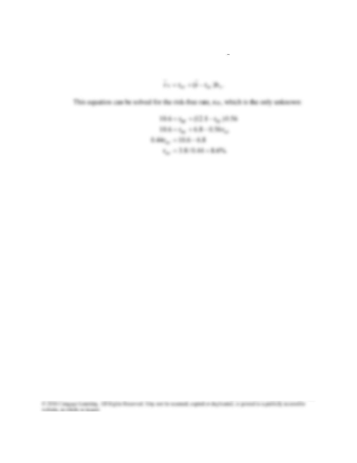
b. The arithmetic average return for Stock X is calculated as follows:

The arithmetic average rate of return on the market portfolio, determined similarly, is

12.1%.

For Stock X, the estimated standard deviation is 13.1 percent:

The standard deviation of returns for the market portfolio is similarly determined to

be 22.6 percent. The results are summarized below:

Stock X Market Portfolio

Answers and Solutions: 3 – 11

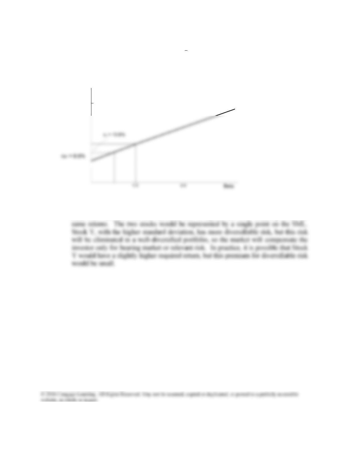
c. Since Stock X is in equilibrium and plots on the Security Market Line (SML), and

given the further assumption that XX rr

  and MM rr 



–and this assumption often

does not hold–then this equation must hold:

Answers and Solutions: 3 – 12

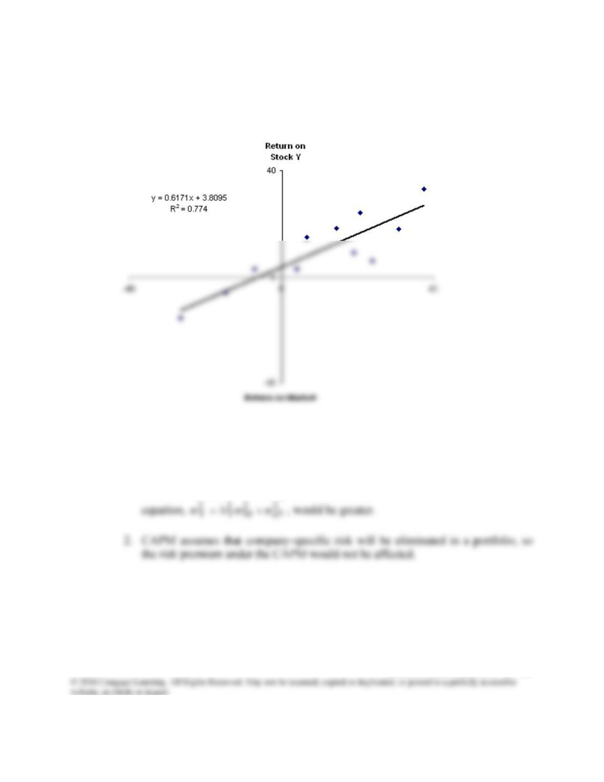
d. The SML is plotted below. Data on the risk-free security (bRF = 0,

rRF = 8.6%) and Security X (bX = 0.56, X

r = 10.6%) provide the two points through

which the SML can be drawn. rM provides a third point.

e. In theory, you would be indifferent between the two stocks. Since they have the same

beta, their relevant risks are identical, and in equilibrium they should provide the

k(%)

20

r(%)

Answers and Solutions: 3 – 13

3-6

a. The regression graph is shown below. Using a spreadsheet, we find b = 0.62.

b. Because b = 0.62, Stock Y is about 62 percent as volatile as the market; thus, its

relative risk is about 62 percent of that of an average firm.

c. 1. Total risk )( 2

Y

 would be greater because the second term of the firm’s risk