
Answers and Solutions: 3 – 14
d. 1. The stock’s variance would not change, but the risk of the stock to an investor
holding a diversified portfolio would be greatly reduced.

Answers and Solutions: 3 – 15
SOLUTION TO SPREADSHEET PROBLEM
3-7 The detailed solution for the spreadsheet problem is available in the file Ch03 P07 Build
Mini Case: 3 – 16
MINI CASE
Answer the following questions.
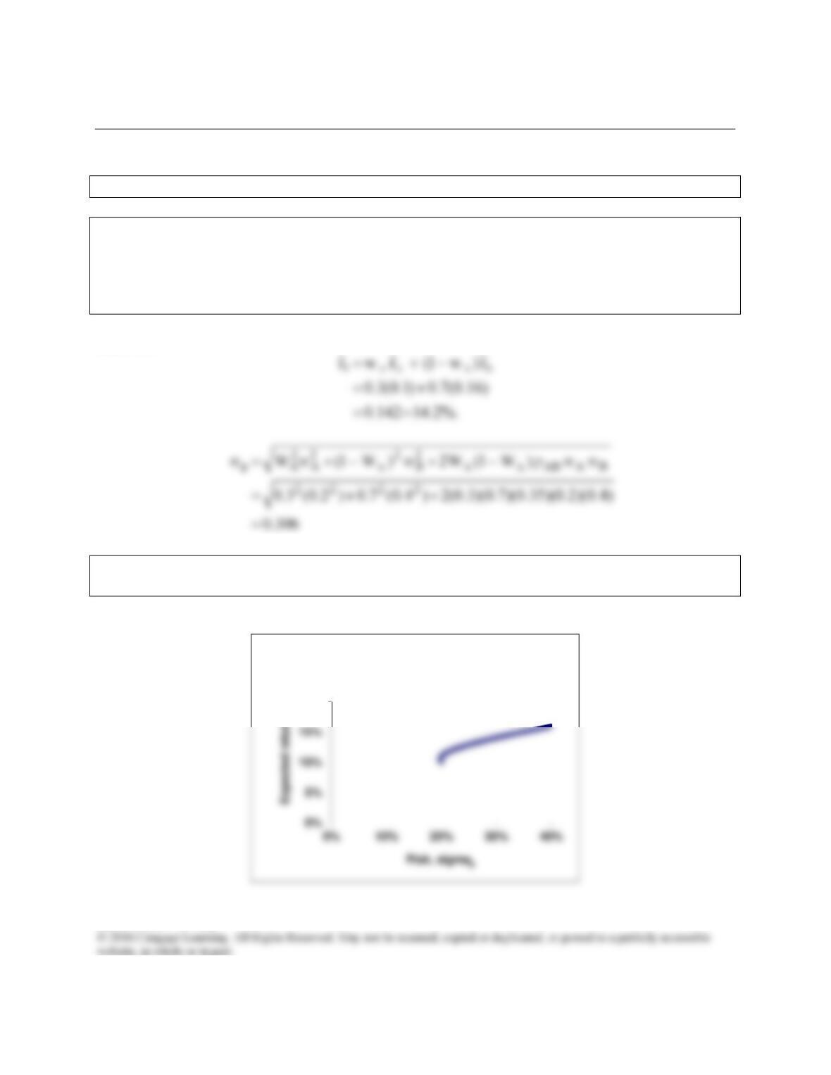
a. Suppose asset A has an expected return of 10 percent and a standard deviation
of 20 percent. Asset B has an expected return of 16 percent and a standard
deviation of 40 percent. If the correlation between A and B is 0.35, what are the
expected return and standard deviation for a portfolio comprised of 30 percent
asset A and 70 percent asset B?
Answer:
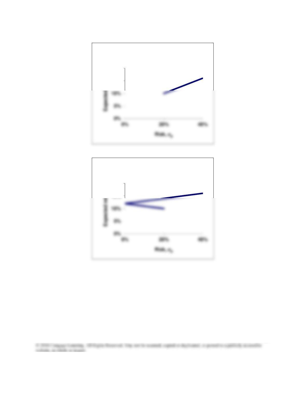
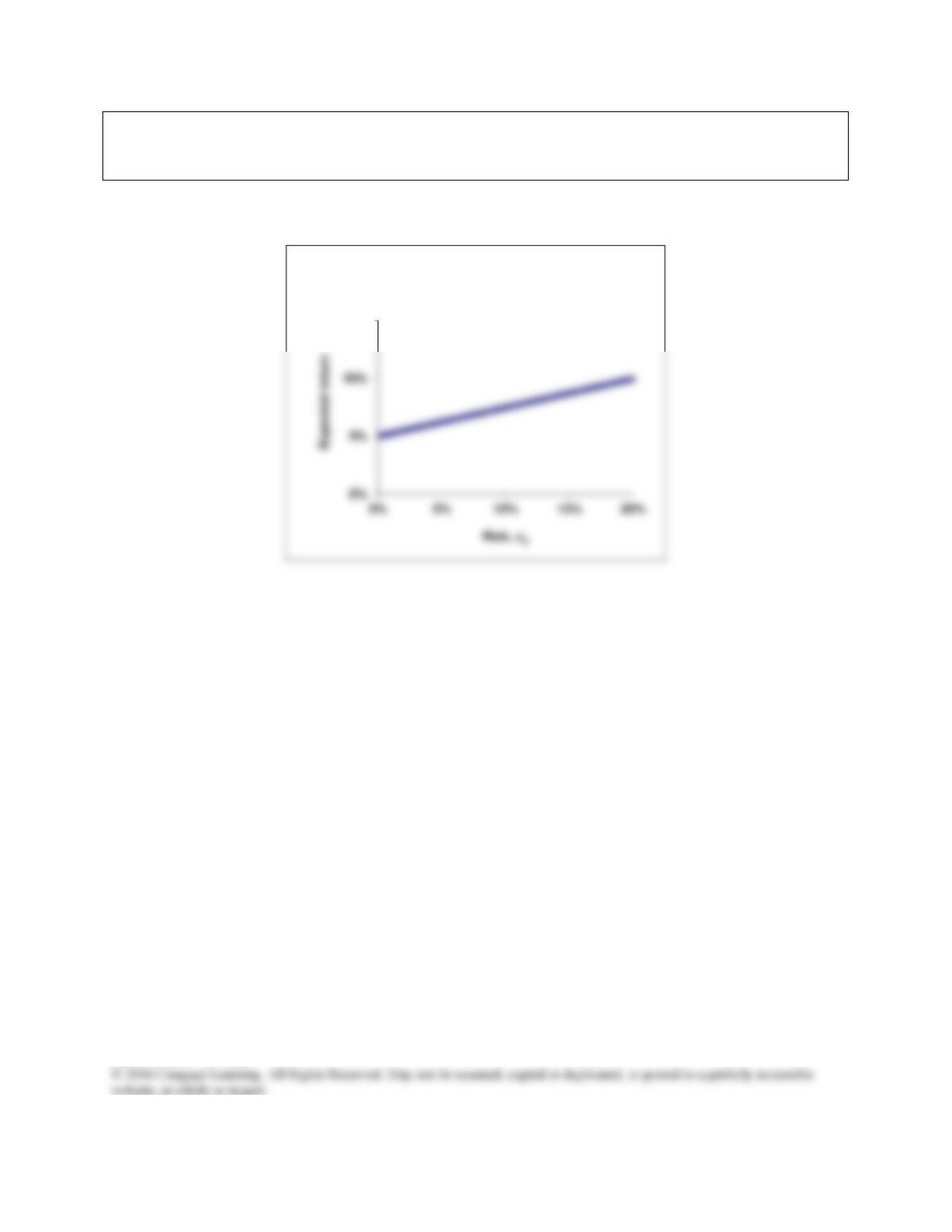
b. Plot the attainable portfolios for a correlation of 0.35. Now plot the attainable
portfolios for correlations of +1.0 and -1.0.
Answer:
20%
pAB = +0.35: Attainable Set of
Risk/Return Combinations
Mini Case: 3 – 17
15%
20%
AB = +1.0: Attainable Set of Risk/Return
Combinations
15%
20%
AB = -1.0: Attainable Set of Risk/Return
Combinations
Mini Case: 3 – 18
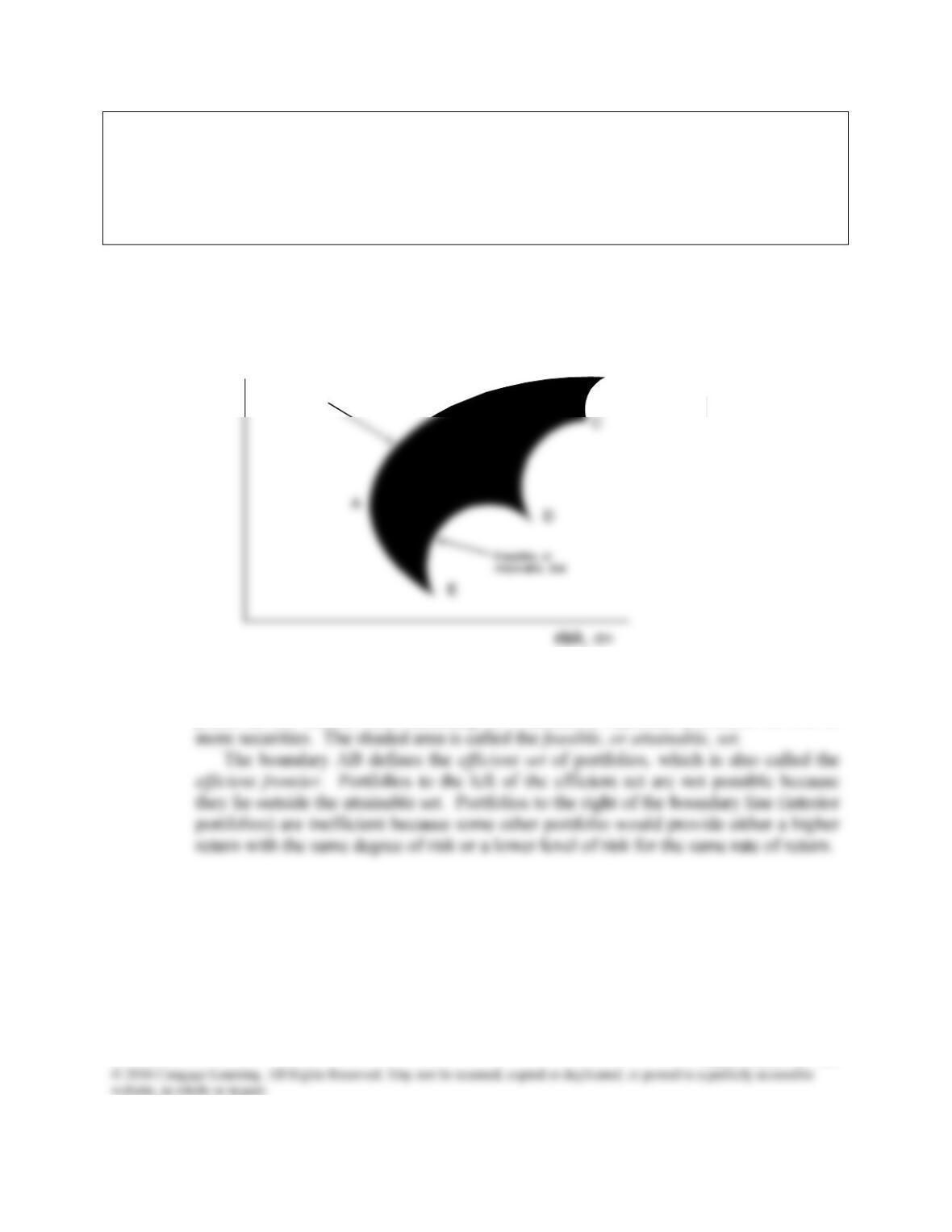
c. Suppose a risk-free asset has an expected return of 5 percent. By definition, its
standard deviation is zero, and its correlation with any other asset is also zero. Using
only asset A and the risk-free asset, plot the attainable portfolios.
Answer:
15%
Attainable Set of Risk/Return
Combinations with Risk-Free Asset
Mini Case: 3 – 19
d. Construct a reasonable, but hypothetical, graph which shows risk, as measured
by portfolio standard deviation, on the x axis and expected rate of return on the
y axis. Now add an illustrative feasible (or attainable) set of portfolios, and show
what portion of the feasible set is efficient. What makes a particular portfolio
efficient? Don’t worry about specific values when constructing the graph—
merely illustrate how things look with “reasonable” data.
Answer:
The figure above shows the feasible set of portfolios. The points B, C, D, and E
represent single securities (or portfolios containing only one security). All the other
points in the shaded area, including its boundaries, represent portfolios of two or
Expected Portfolio
B
Return, kp
Efficient Set
(A,B)
^
Expected Portfolio
Return
^
rP
Mini Case: 3 – 20
e. Now add a set of indifference curves to the graph created for part B. What do
these curves represent? What is the optimal portfolio for this investor? Finally,
add a second set of indifference curves which leads to the selection of a different
optimal portfolio. Why do the two investors choose different portfolios?
Answer:
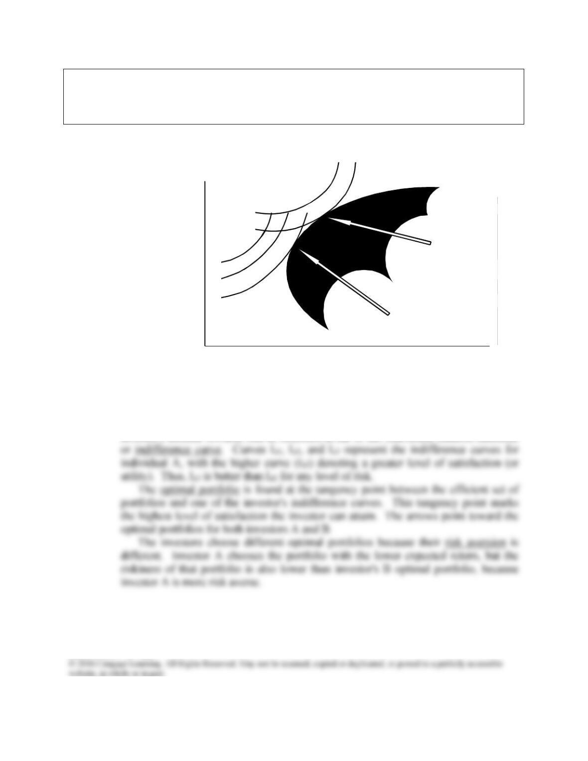
The figure above shows the indifference curves for two hypothetical investors, A and
B. To determine the optimal portfolio for a particular investor, we must know the
investor’s attitude towards risk as reflected in his or her risk/return tradeoff function,
Expected Portfolio
Risk,
p
A
B
C
D
E
IA3
IA2
IA1
IB2
IB1
Optimal
Portfolio
Investor B
Optimal
Portfolio
Investor A
Return, kp
^
Expected Portfolio
Return,
^
rp
risk, P

Mini Case: 3 – 21
f. What is the capital asset pricing model (CAPM)? What are the assumptions
that underlie the model?
Answer: The Capital Asset Pricing Model (CAPM) is an equilibrium model which specifies
the relationship between risk and required rates of return on assets when they are held
in well-diversified portfolios. The CAPM requires an extensive set of assumptions:
All investors are single-period expected utility of terminal wealth maximizers,
Mini Case: 3 – 22
g. Now add the risk-free asset. What impact does this have on the efficient
frontier?
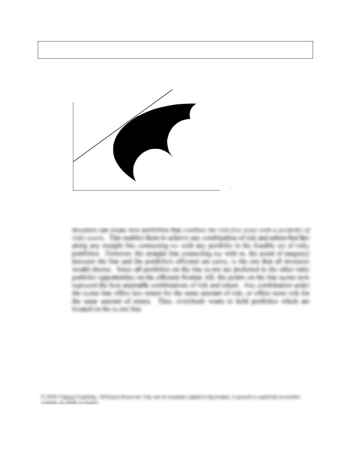
Answer: The risk-free asset by definition has zero risk, and hence σ = 0%, so it is plotted on
the vertical axis. Now, given the possibility of investing in the risk-free asset,
Expected Portfolio
Risk,
p
A
B
Z
M
kRF
Return, kp
^
Expected Portfolio
Return,
^
rp
rR
σp
Mini Case: 3 – 23
h. Write out the equation for the capital market line (CML) and draw it on the
graph. Interpret the CML. Now add a set of indifference curves, and illustrate
how an investor’s optimal portfolio is some combination of the risky portfolio
and the risk-free asset. What is the composition of the risky portfolio?
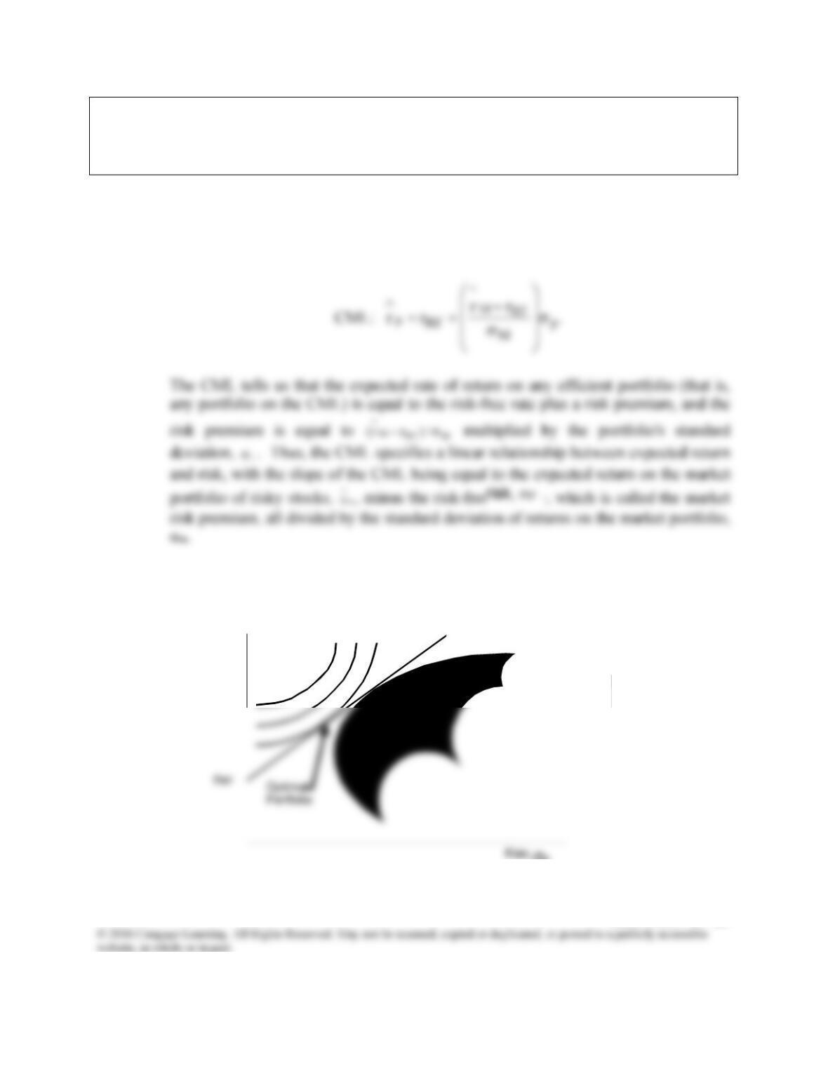
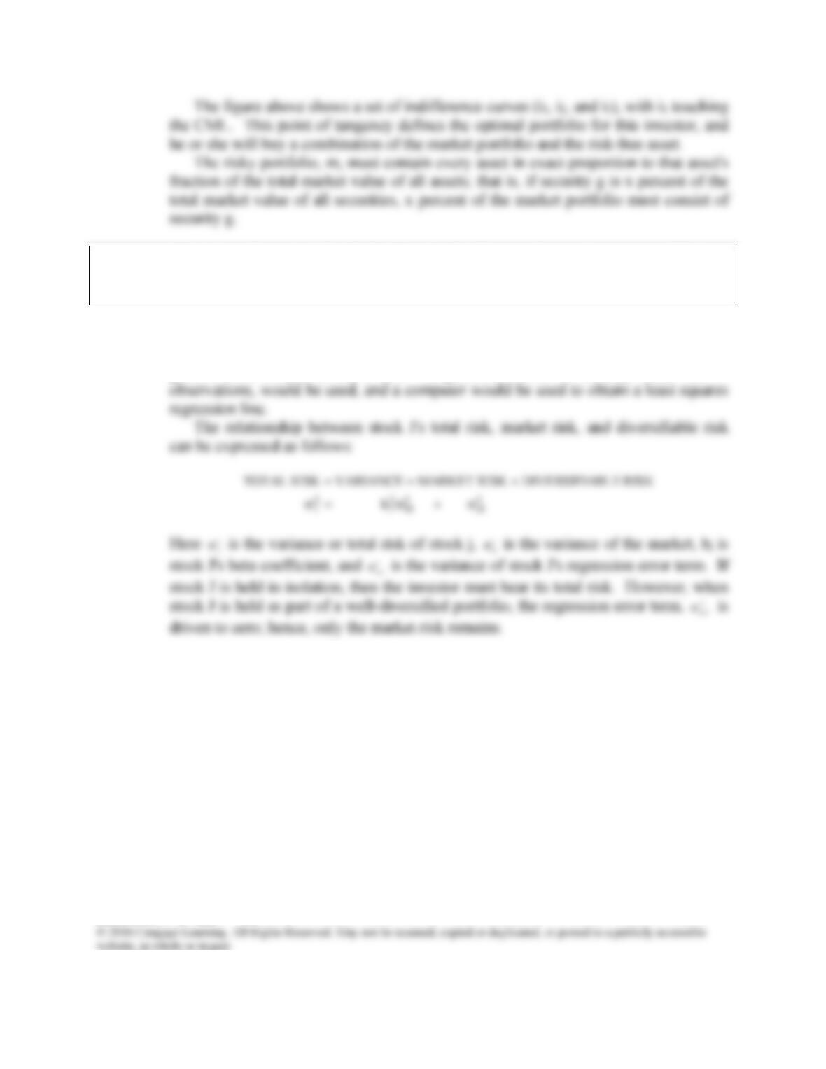
Answer: The line rRFmz in the figure above is called the capital market line (CML). It has an
intercept of rRF and a slope of MRF
M/)rr(
. Therefore the equation for the capital
market line may be expressed as follows:
Expected Rate
CML
I3I2I1
p
of Return, kp
^
Expected Rate
of Return,
^
rp
σp
Mini Case: 3 – 24
i. What is a characteristic line? How is this line used to estimate a stock’s beta
coefficient? Write out and explain the formula that relates total risk, market
risk, and diversifiable risk.
Answer: Betas are calculated as the slope of the characteristic line, which is the regression line
formed by plotting returns on a given stock on the y axis against returns on the
general stock market on the x axis. In practice, 5 years of monthly data, with 60
Mini Case: 3 – 25
j. What are two potential tests that can be conducted to verify the CAPM? What
are the results of such tests? What is roll’s critique of CAPM tests?
Answer: Since the CAPM was developed on the basis of a set of unrealistic assumptions,
empirical tests should be used to verify the CAPM. The first test looks for stability in
historical betas. If betas have been stable in the past for a particular stock, then its
The second type of test is based on the slope of the SML. As we have seen, the
CAPM states that a linear relationship exists between a security’s required rate of
return and its beta. Further, when the SML is graphed, the vertical axis intercept
should be rRF, and the required rate of return for a stock (or portfolio) with beta = 1.0
should be rm, the required rate of return on the market. Various researchers have
Roll questioned whether it is even conceptually possible to test the CAPM. Roll
showed that the linear relationship which prior researchers had observed in graphs
resulted from the mathematical properties of the models being tested, hence that a
finding of linearity proved nothing about the validity of the CAPM. Roll’s work did
Mini Case: 3 – 26
k. Briefly explain the difference between the CAPM and the arbitrage pricing
theory (APT).
Answer: The CAPM is a single-factor model, while the Arbitrage Pricing Theory (APT) can
include any number of risk factors. It is likely that the required return is dependent
on many fundamental factors such as the GNP growth, expected inflation, and