
SOLUTION TO SPREADSHEET PROBLEM
29-23 The detailed solution for the spreadsheet problem is available in the file Solution for
IFM10 Ch 29 P23 Build a Model.xls on the textbook’s web site..
Answers and Solutions: 29 – 20
MINI CASE
Susan Greene is a financial planner. Her job is to suggest and implement investment and
savings plans for clients, some of whom are of modest means and some of whom are quite
wealthy. Last month a Fortune 500 firm contracted with Susan’s firm to provide financial
planning services to all 150 of its middle level managers over a 3–month period. Susan’s plan is
first to conduct an hour–long seminar to provide some general information about investments
and their risks, and then to arrange individual meetings for follow–up. She has asked you to
help her with the seminar by working out some examples to illustrate savings and investment
plans, and to prepare some information about the risks and rewards of investments in common
stock. She particularly wants you to explain how risk and return are related. Please answer
the following questions and prepare the following illustrations for her.
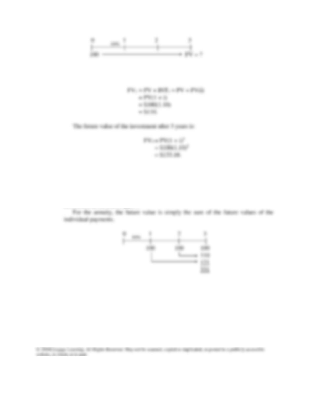
a. Draw time lines (1) for a $100 lump sum due at the end of year 2 and
(2) for a 3-year $100 annuity. Explain how each investment of $100 grows to its
future value after 3 years if the interest rate is 10 percent.
Answer: A time line is a graphical representation which is used to show the timing of cash flows.
The tick marks represent end of periods (often years), so time 0 is today; time 1 is the end
of the first year, or 1 year from today; and so on.
Mini Case: 29 – 21
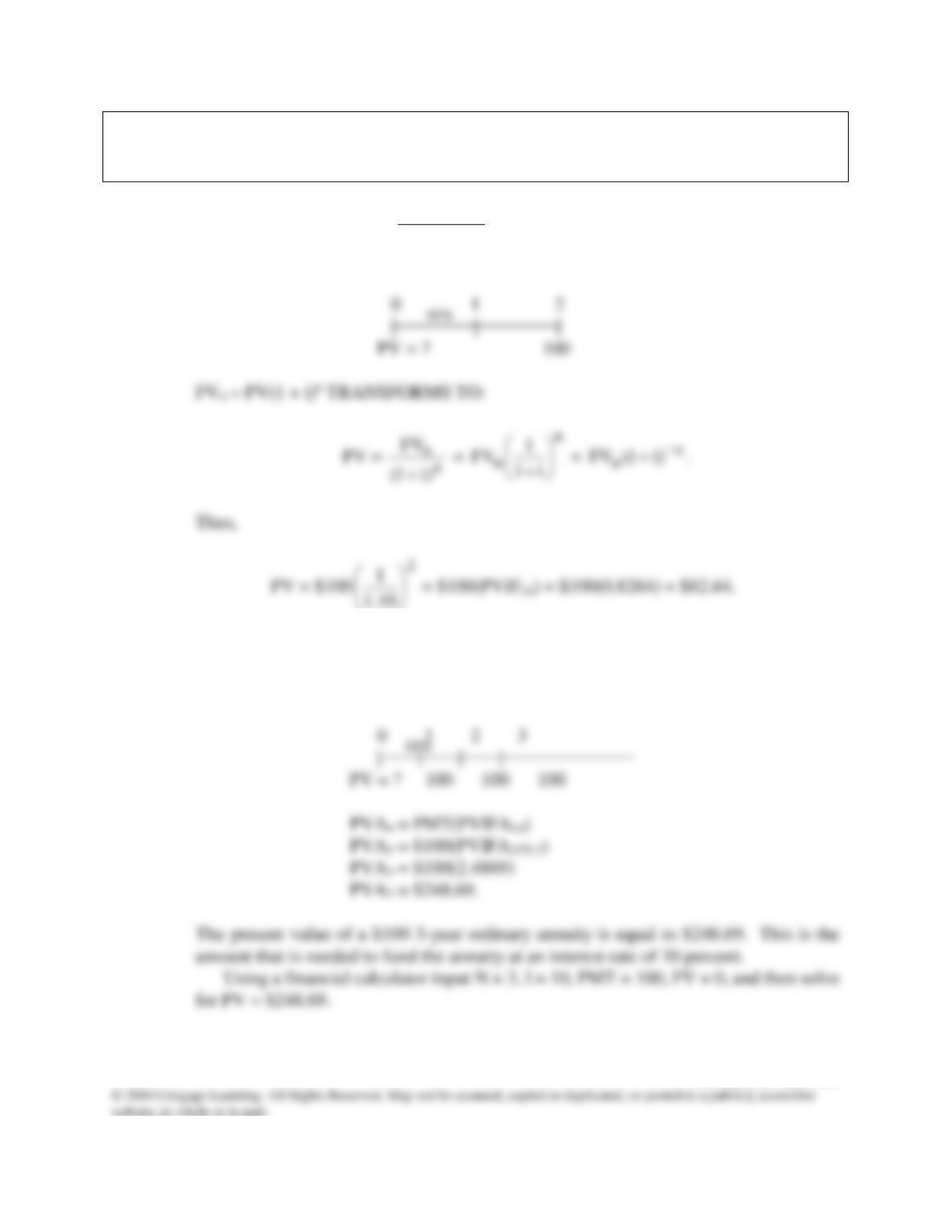
Finding future values, or moving to the right on a time line, is called compounding.
The future value of a $100 investment after 1 year is:
In general,
FVn = PV(1 + i)n.
The future value of $100 received in year 2 at year 3 is simply the future value of a $100
investment at the end of year 1.
Mini Case: 29 – 22
b. What is the present value of the $100 lump sum due at the end of 2 years and the 3–
year, $100 annuity in part a? How much would you need to invest in an account
that earns 10 percent in order to fund this annuity?
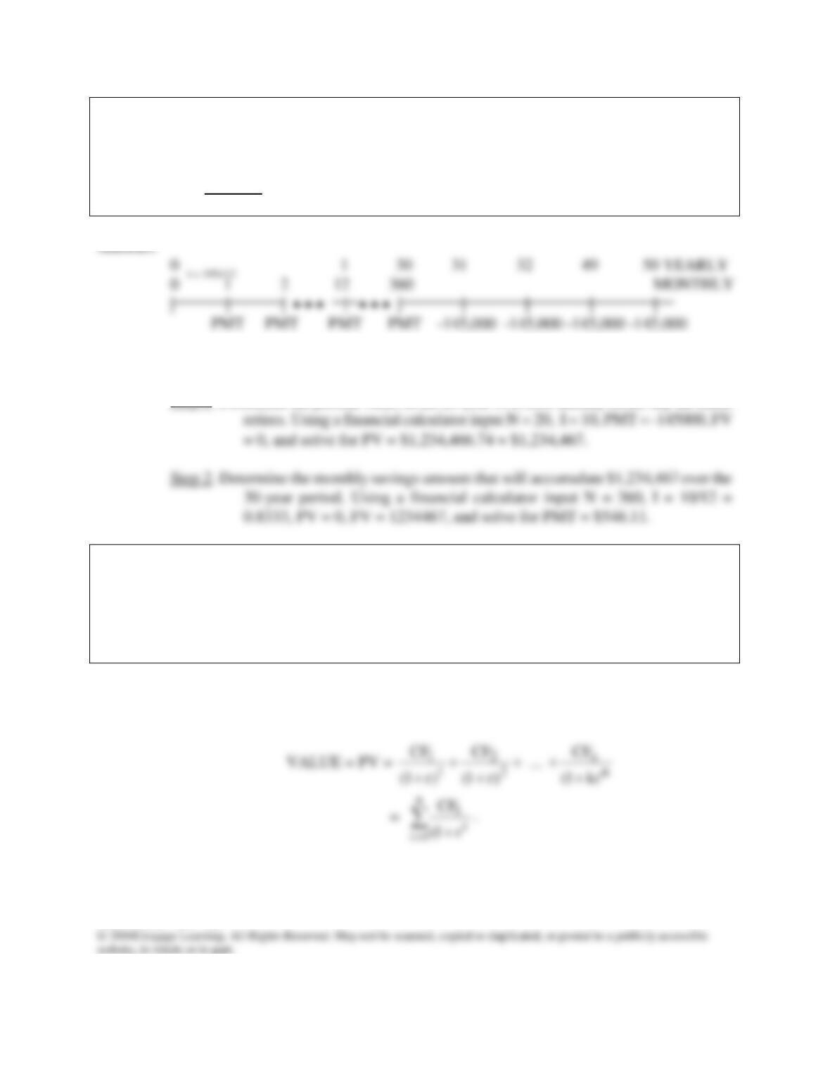
Answer: Finding present values, or discounting (moving to the left along the time line), is the
reverse of compounding. The basic present value equation is the reciprocal of the
compounding equation:
The same methods used for finding future values are also used to find present values.
Using a financial calculator input N = 2, I = 10, PMT = 0, FV = 100, and then solve
for PV = $82.64.
Mini Case: 29 – 23
c. If inflation is 3 percent per year, then an annual salary of $60,000 today will rise to
about $145,000 in 30 years. One of Susan’s clients wants to maintain a purchasing
power of $60,000 in today’s dollars, at least for the first year of retirement, so she is
planning to draw $145,000 a year at year end after retirement. How much must she
save monthly to retire in 30 years and draw an annual pension of $145,000 for 20
years after retirement? Assume a 10 percent per year return on investments.
This problem needs to be solved in two steps.
Step 1. Determine the present value of the 20–year $145,000 annuity on the day the client
d. Susan has also asked you to prepare some information about various investments
that might be used to meet these retirement goals. To do this you will need to
discuss not only how bonds and stocks are priced but also the concept of the trade–
off between risk and return. To begin, describe the key features of a bond and
show how its value is determined. Find the value of a 10-year, $1,000 par value
bond with a 10 percent annual coupon and a required rate of return of 10 percent.
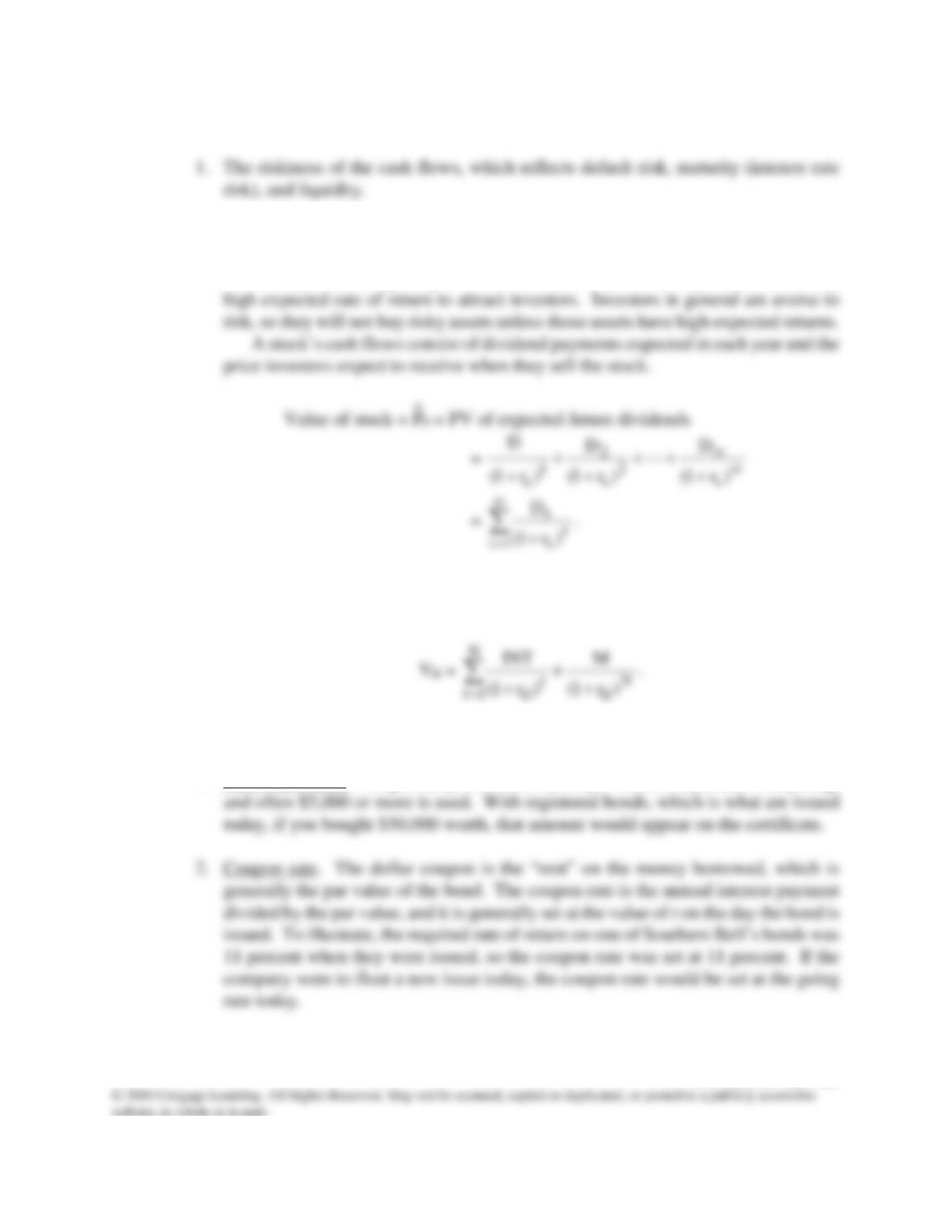
Answer: The value of any asset can be found as the present value of its expected future cash flows,
CFt, discounted at the rate r:
Mini Case: 29 – 24
The discount rate depends on:
2. The general level of interest rates, which reflects inflation, supply of and demand for
money, production opportunities, and time preferences for consumption.
An asset with a high degree of relevant (market) risk must provide a relatively
A bond’s cash flows consist of periodic interest payments and a lump sum
principal amount due in the future.
Key features of a bond:
1. Par or face value. We generally assume a $1,000 par value, but par can be anything,
Mini Case: 29 – 25
3. Maturity. This is the number of years until the bond matures and the issuer must
repay the loan (return the par value). The Southern Bell bonds had a 30–year maturity
when they were issued, but the maturity declines by 1 year each year after their issue.
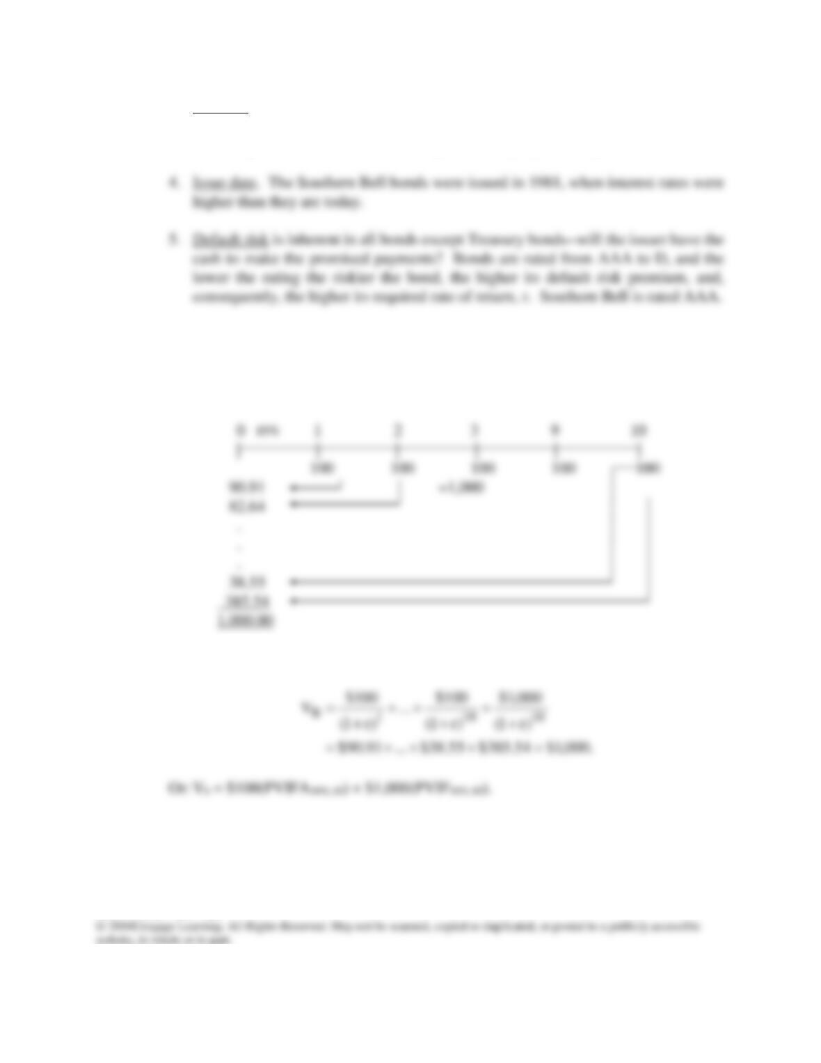
A bond has a specific cash flow pattern consisting of a stream of constant interest
payments plus the return of par at maturity. The annual coupon payment is the cash flow:
pmt = (coupon rate) × (par value) = 0.1($1,000) = $100.
For a 10-year, 10 percent annual coupon bond, the bond’s value is found as follows:
Expressed as an equation, we have:
Mini Case: 29 – 26
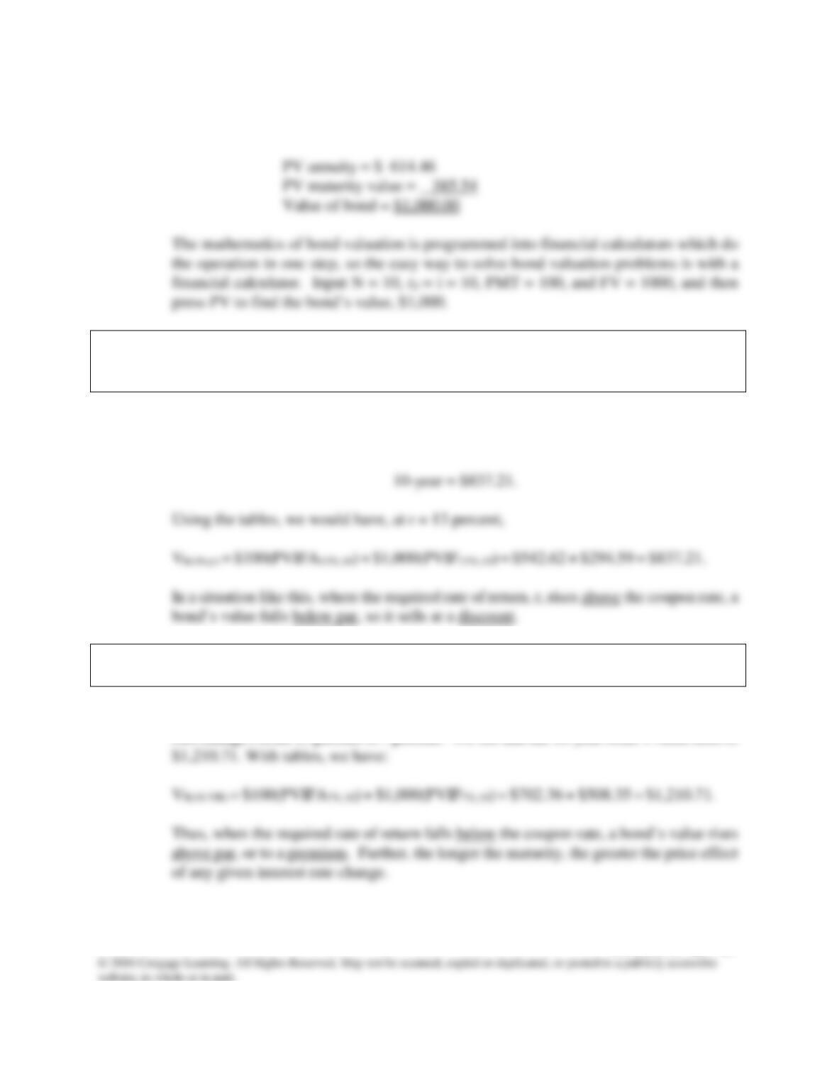
The bond consists of a 10-year, 10 percent annuity of $100 per year plus a $1,000 lump
sum payment at t = 10:
e. 1. What would be the value of the bond described in part d if, just after it had been
issued, the expected inflation rate rose by 3 percentage points, causing investors to
require a 13 percent return?
Answer: With a financial calculator, just change the value of r = i from 10 percent to 13 percent,
and press the PV button to determine the value of the bond:
e. 2. What would happen to the bond’s value if inflation fell, causing rd to decline to 7
percent?
Answer: In the second situation, where r falls to 7 percent, the price of the bond rises above par.
Just change r from 13 percent to 7 percent. We see that the 10-year bond’s value rises to
Mini Case: 29 – 27
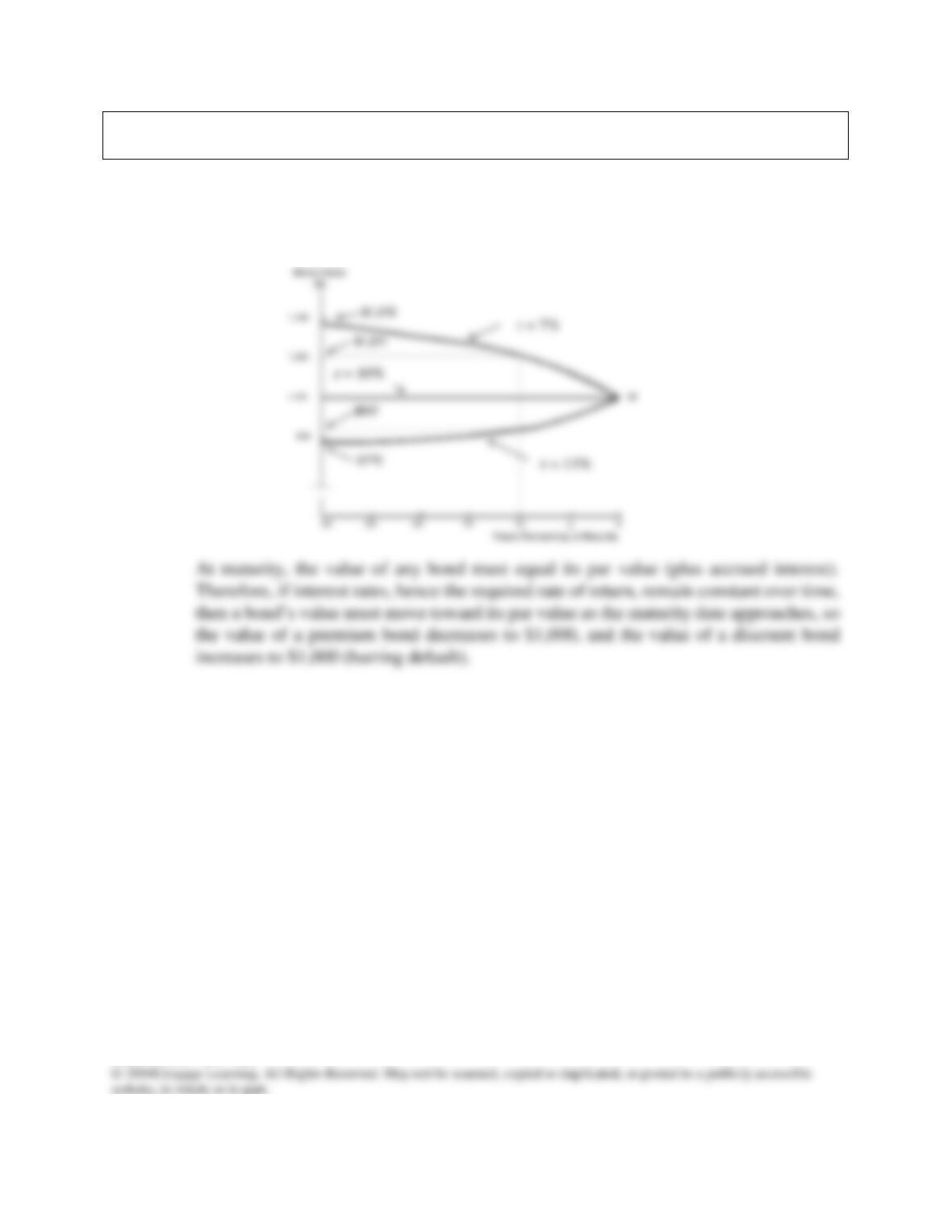
e. 3. What would happen to the value of the 10–year bond over time if the required rate
of return remained at 13 percent? If it remained at 7 percent?
Answer: Assuming that interest rates remain at the new levels (either 7 percent or 13 percent), we
could find the bond’s value as time passes, and as the maturity date approaches. If we
then plotted the data, we would find the situation shown below:
Mini Case: 29 – 28
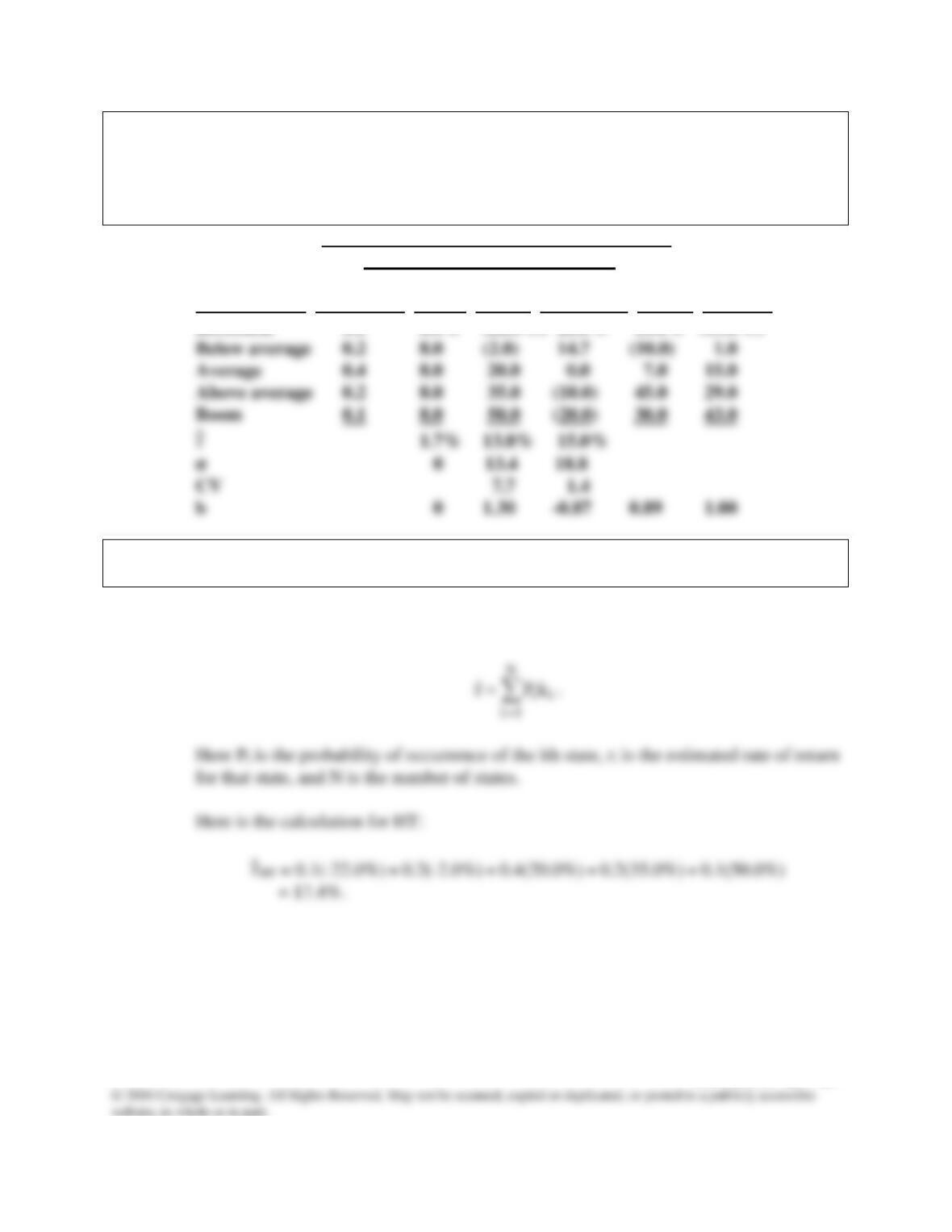
f. As an alternative to bond investments, susan wants you to present some data on
stock investments. The following table has the returns that should occur under
various states of the economy for a variety of assets. Some of the output variables
have been calculated, but blanks are shown for others.
Estimated rate of return
Stocks
State of market
The economy probability T-bills HT Collections USR portfolio
Recession 0.1 8.0% (22.0%) 28.0% 10.0% (13.0%)
1. Calculate the expected return, standard deviation, and CV for HT and the T–bills.
Answer: The expected rate of return, ^
r, is expressed as follows:
Mini Case: 29 – 29
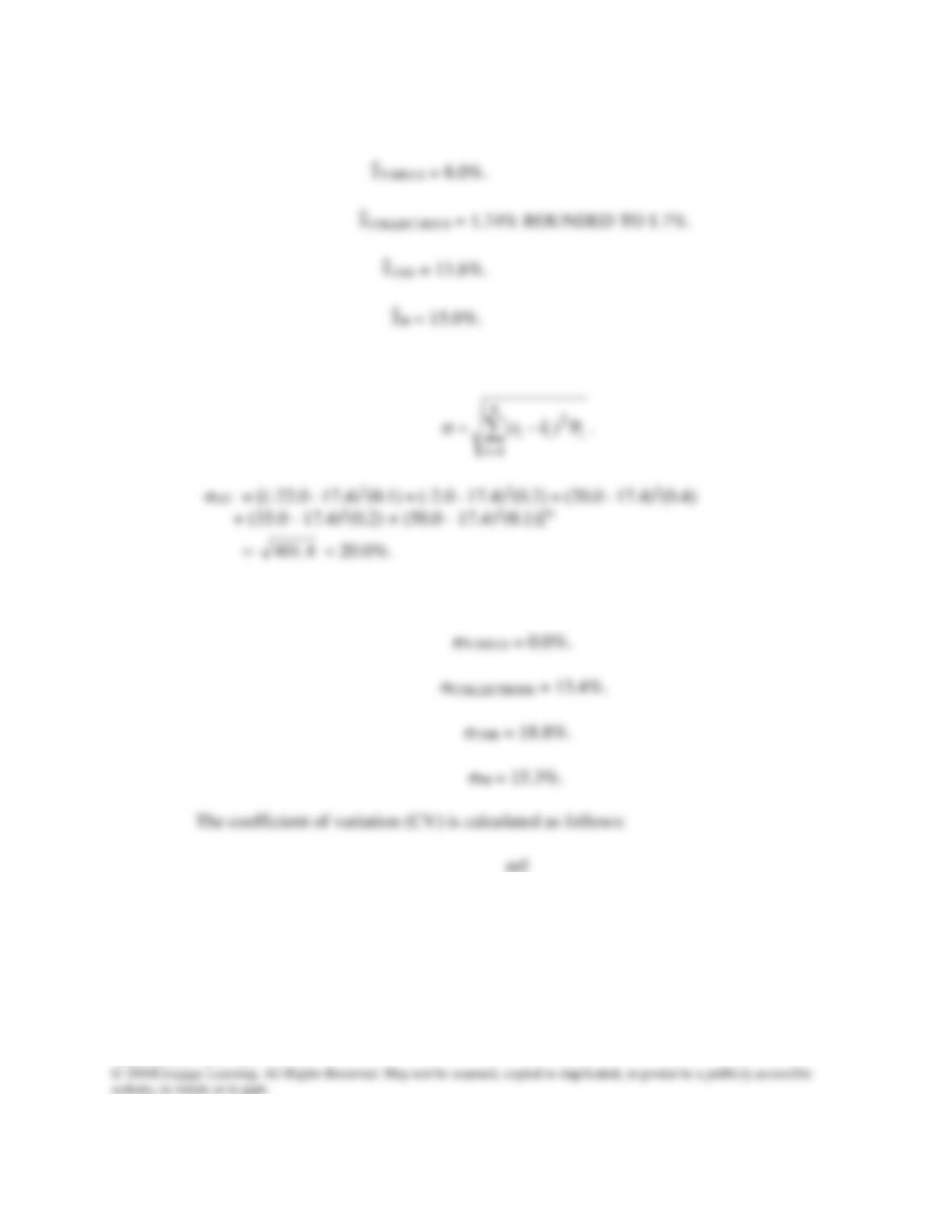
We use the same formula to calculate r for the other alternatives:
The standard deviation is calculated as follows:
Here are the standard deviations for the other alternatives:
Mini Case: 29 – 30
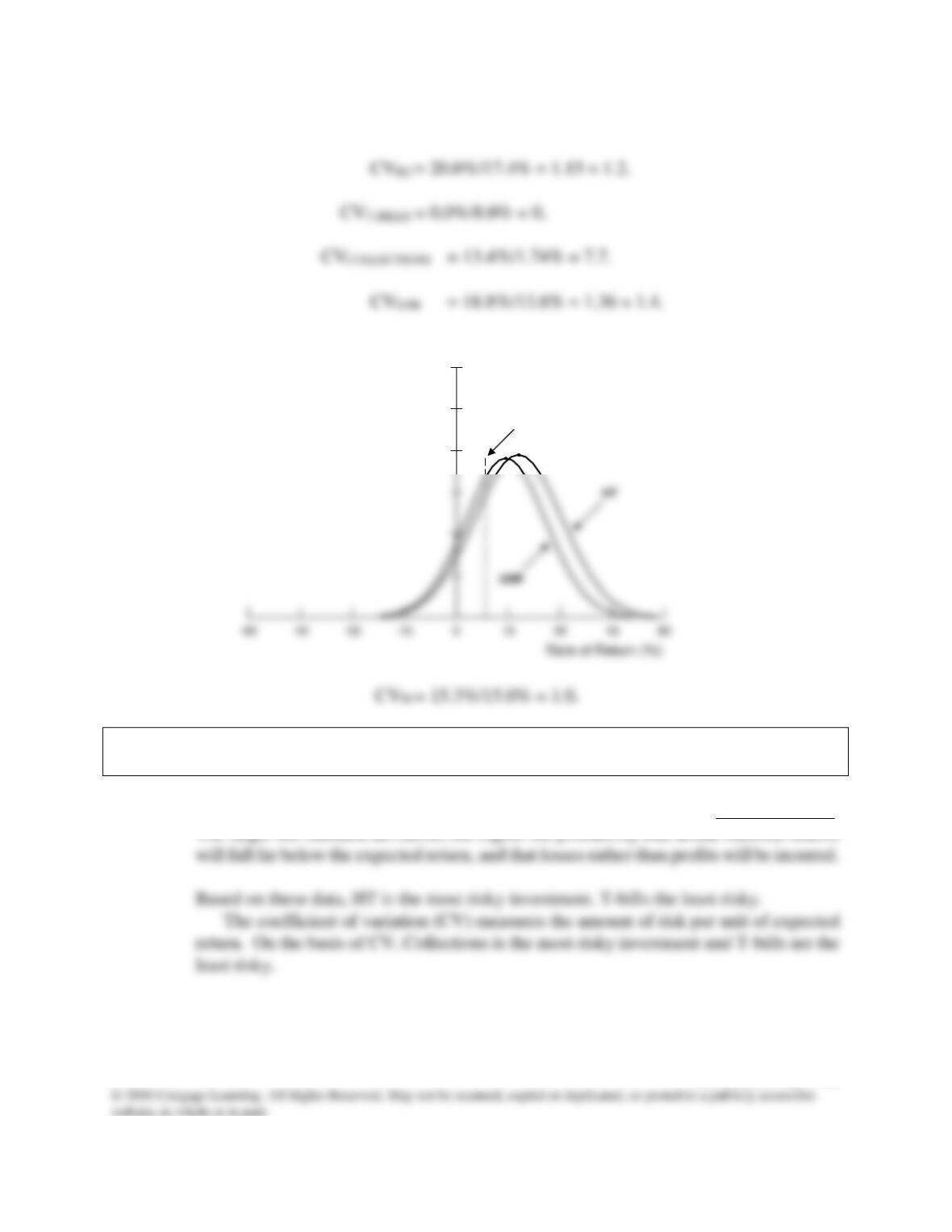
Here are the CVs:
f. 2. How do HT’s expected return, standard deviation, and CV compare with those of
the other assets, and what are the implications of these comparisons?
Answer: The standard deviation is a measure of a security’s (or a portfolio’s) stand–alone risk.
Probability of
Occurrence
T-Bills
Mini Case: 29 – 31
g. Suppose you created a 2–stock portfolio by investing $50,000 in ht and $50,000 in
Collections.
1. Calculate the expected return (^
rP), the standard deviation (σP), coefficient of
variation (CVP), and beta (bP) for this portfolio.
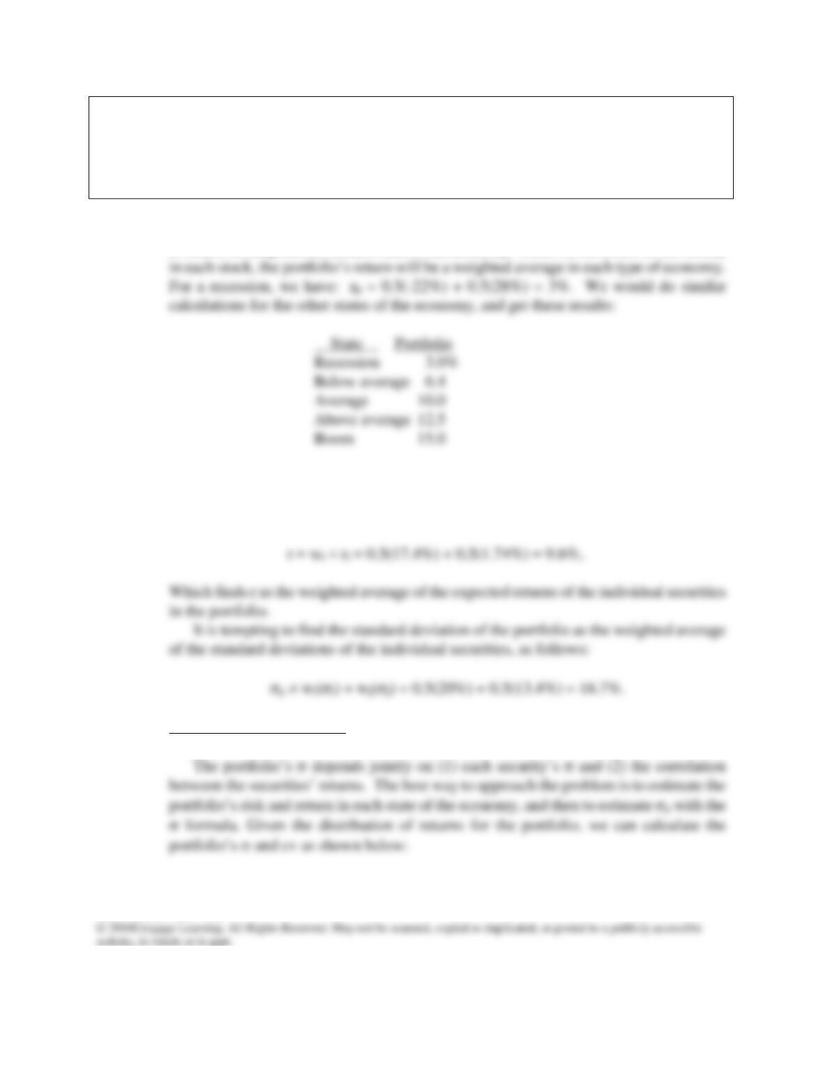
Answer: To find the expected rate of return on the two-stock portfolio, we first calculate the rate
of return on the portfolio in each state of the economy. Since we have half of our money
Now we can multiply probabilities times outcomes in each state to get the expected
return on this two-stock portfolio, 9.6 percent.
Alternatively, we could apply this formula,
However, this is not correct—it is necessary to use a different formula, the one for σ that
we used earlier, applied to the two-stock portfolio’s returns.
Mini Case: 29 – 32
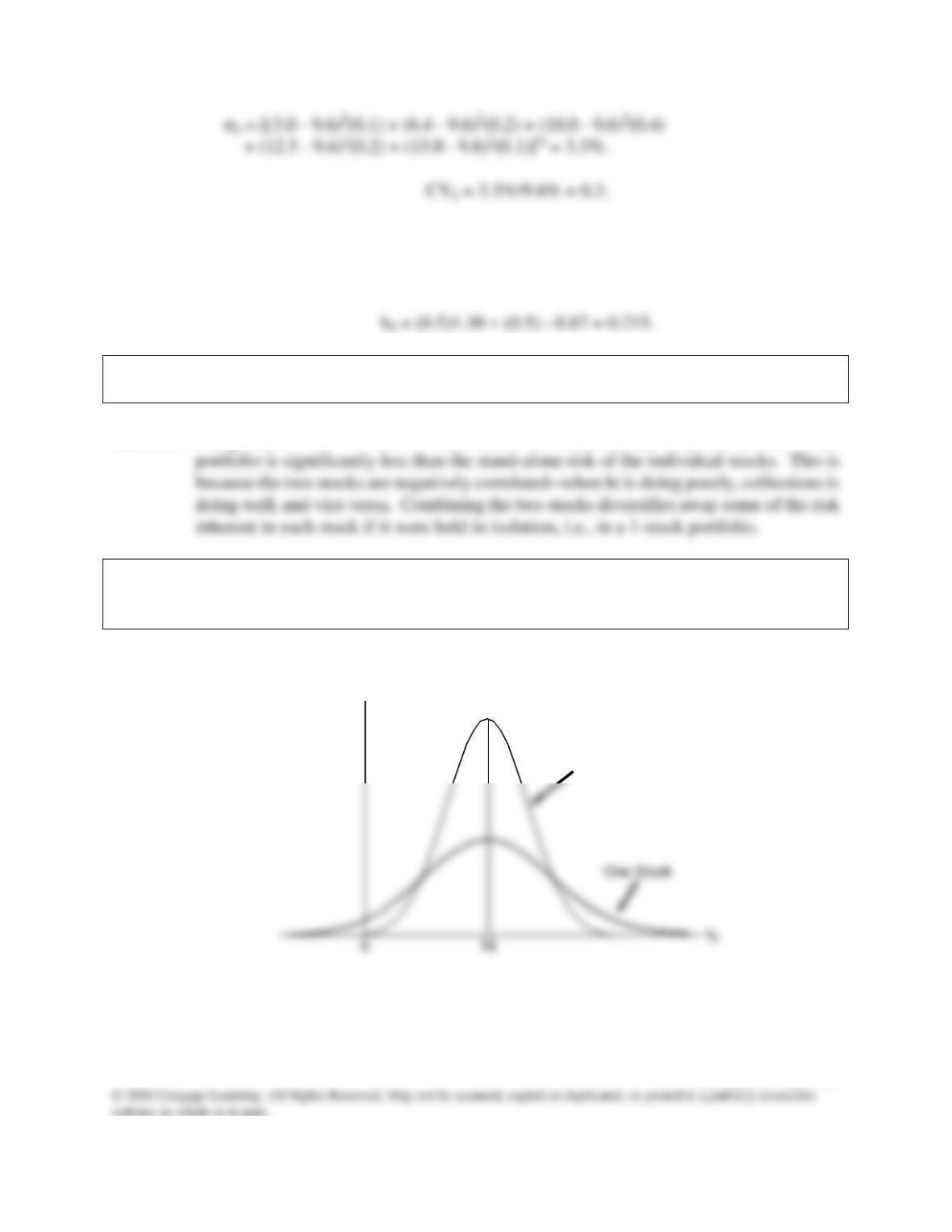
The portfolio’s beta is a weighted average of the individual assets’ betas. Thus, for a
portfolio consisting of 50 percent ht and 50 percent collections the portfolio’s beta is
calculated as:
g. 2. How does the riskiness of this portfolio compare to the riskiness of the individual
stocks if held in isolation?
Answer: Using either σ or CV as our stand-alone risk measure, the stand–alone risk of the
h. Explain what happens to the risk and expected return on a portfolio constructed
from randomly picked stocks if we start with a 1–stock portfolio and add more and
more stocks.
ANSWER:
Density
Portfolio of Stocks
with k
P
= 16%
Portfolio of Stocks
with rP = 16%
Mini Case: 29 – 33
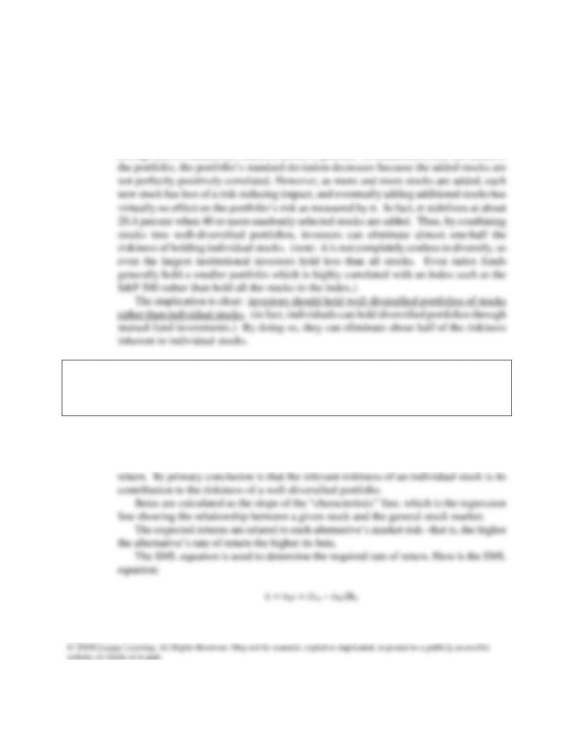
The standard deviation gets smaller as more stocks are combined in the portfolio, while rp
(the portfolio’s return) remains constant. Thus, by adding stocks to your portfolio, which
initially started as a 1-stock portfolio, risk has been reduced.
In the real world, stocks are positively correlated with one another—if the economy
does well, so do stocks in general, and vice versa. Correlation coefficients between
stocks generally range from +0.5 to +0.7. A single stock selected at random would on
average have a standard deviation of about 35 percent. As additional stocks are added to
i. How are risk and return related under the CAPM? Specifically, how is beta
calculated and how are required rates of return determined? Use the SML to
calculate required rates of return for the three stocks in Part F. How do these
required returns compare with the stocks’ expected returns?
Answer: We know that investors demand a premium for bearing risk; that is, the higher the
riskiness of a security, the higher its expected return must be to induce investors to buy
(or to hold) it. The CAPM is used to analyze the relationship between risk and rates of
Mini Case: 29 – 34
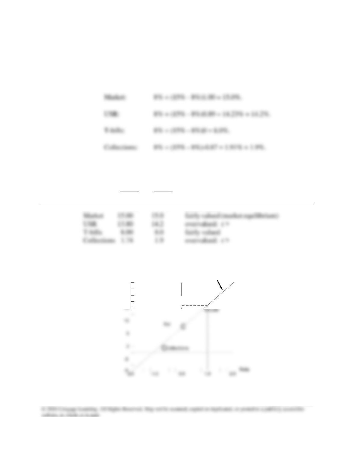
If we use the T-bill yield as a proxy for the risk–free rate, then rRF = 8%. Further, our
estimate of rM = ^
rM is 15 percent. Thus, the required rates of return for the alternatives
are as follows:
HT: 8% + (15% – 8%)1.30 = 17.10%.
We have the following relationships:
Expected Required
Return Return
Security (^
r) (r) Condition
HT 17.40% 17.1% undervalued: > r
22
18
Required and Expected
Rates of Return (%)
HT
SML: k
i
= k
RF
+ (k
M
– k
RF
)b
i
k
M
C
C
= 8% + 7%(b
i
)
SML: r
i
= r
RF
+ (r
i
– r
RF
)b
i
= 8% + 7% bi
r
M
Mini Case: 29 – 35
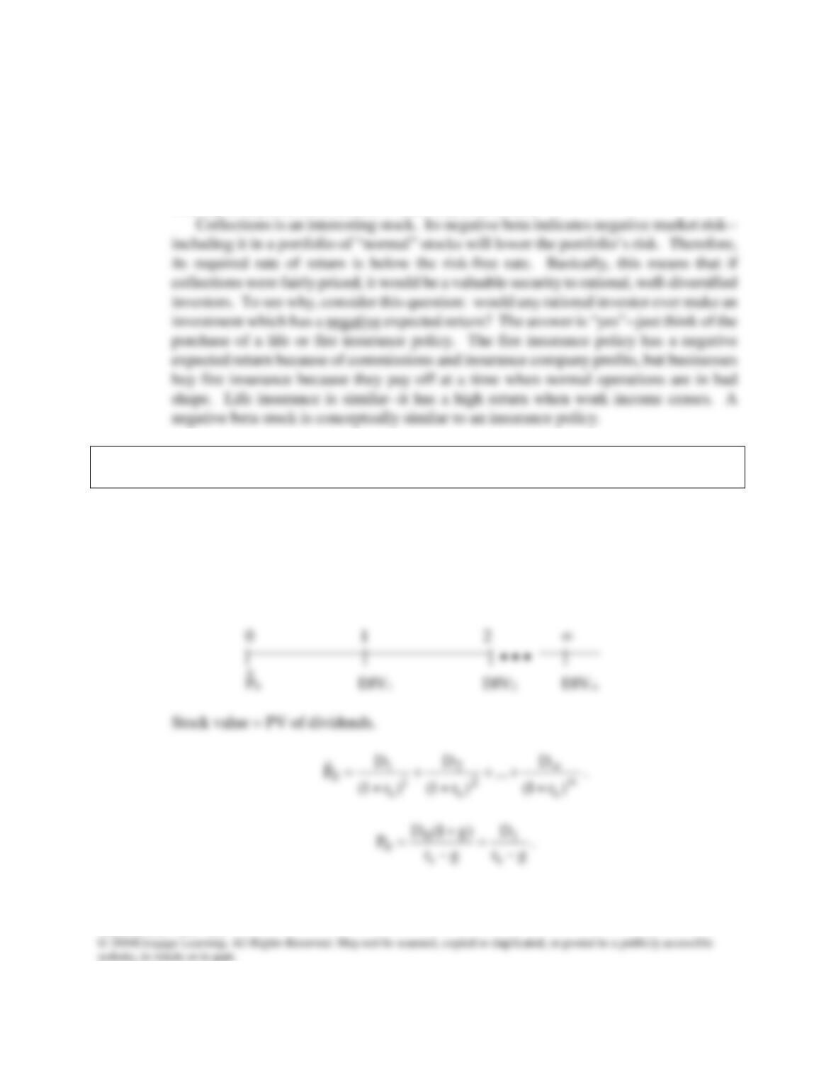
(Note: The plot looks somewhat unusual in that the x–axis extends to the left of zero.
We have a negative beta stock, hence a required return that is less than the risk–free rate.)
The T–bills and market portfolio plot on the SML, HT plots above it, and collections and
usr plot below it. Thus, the T-bills and the market portfolio promise a fair return, HT is a
good deal because it has an expected return above its required return, and collections and
USR have expected returns below their required returns.
j. Explain why the price of a share of stock is calculated as the present value of its
expected future dividends, using a time line to help with your explanation.
Answer: common stocks provide an expected future cash flow stream, and a stock’s value is found
in the same manner as the values of other financial assets—namely, as the present value of
the expected future cash flow stream. The expected cash flows consist of two elements:
(1) the dividends expected in each year and (2) the price investors expect to receive when
they sell the stock.
Mini Case: 29 – 36
k. One of Susan’s clients has just inherited some stock of a company named bon
temps, and he asked her to evaluate the stock for him. Use the dividend growth
model to find the price of a share of Bon Temps stock. Bon Temps has a beta
coefficient of 1.2, the risk-free rate is 7 percent, the required rate of return on the
market is 12 percent. Bon Temps is a constant growth firm whose last dividend
(D0) was $2 and whose dividend is expected to grow at a rate of 6 percent
indefinitely.
Answer: Bon Temps is a constant growth stock, and its dividend is expected to grow at a constant
rate of 6 percent per year. Use the SML to calculate rs:
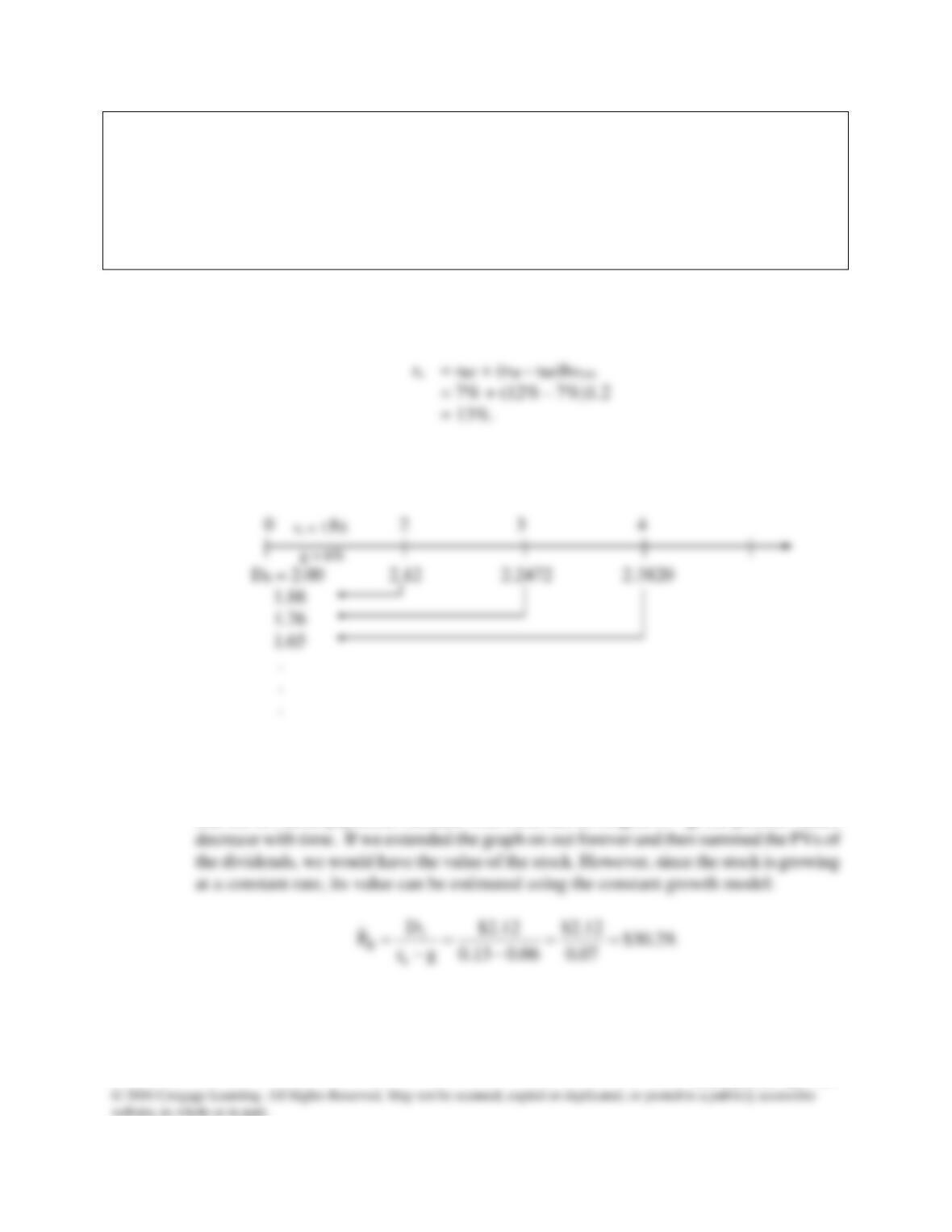
Expressed as a time line, we have the following setup. Just enter 2 in your calculator;
then keep multiplying by 1 + g = 1.06 to get D1, D2, and D3:
We could extend the time line on out forever, find the value of Bon Temps’ dividends
for every year on out into the future, and then the PV of each dividend, discounted at r =
13%. For example, the PV of D1 is $1.8761; the PV of D2 is $1.7599; and so forth. Note
that the dividend payments increase with time, but as long as rs > g, the present values
Mini Case: 29 – 37
l. If Bon Temps were selling for $30.29, what would be its implied expected rate of
return?
Answer: The constant growth model can be rearranged to this form:
m. Now assume that bon temps is expected to experience supernormal growth of 30
percent for the next 3 years, then to return to its long–run constant growth rate of 6
percent. What is the stock’s value under these conditions?
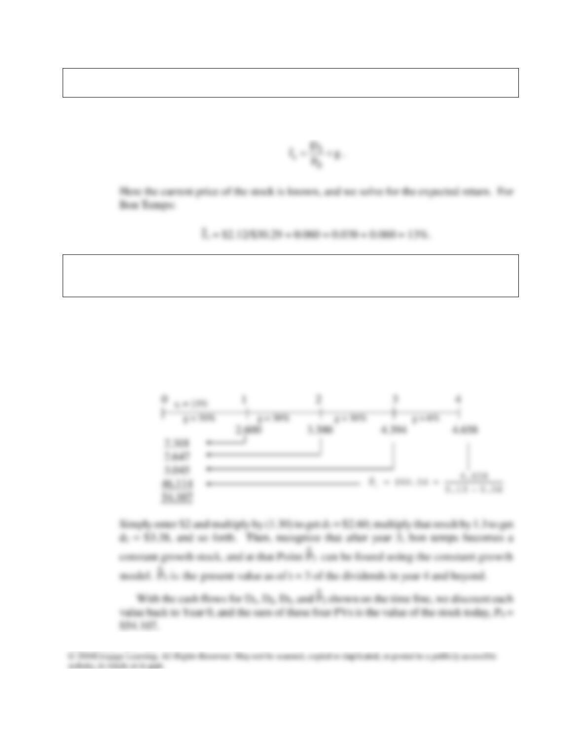
Answer: Bon Temps is no longer a constant growth stock, so the constant growth model is not
applicable. Note, however, that the stock is expected to become a constant growth stock
in 3 years. Thus, it has a nonconstant growth period followed by constant growth. The
easiest way to value such nonconstant growth stocks is to set the situation up on a time
line as shown below:
Mini Case: 29 – 38