1
2
3
4
5
6
7
8
9
10
11
12
13
14
15
16
17
18
19
20
23
24
25
26
27
28
29
30
31
· All values are known with certainty and constant over time.
· All carrying costs are variable, so carrying costs change proportionally with changes in inventory levels
These assumed conditions are not met in the real world, and, as a result, safety stocks are carried, and these stocks raise
· All ordering costs are fixed per order; that is, the company pays a fixed amount to order and receive each shipment of
32
33
34
35
36
37
38
39
40
41
42
44
45
46
47
48
49
50
51
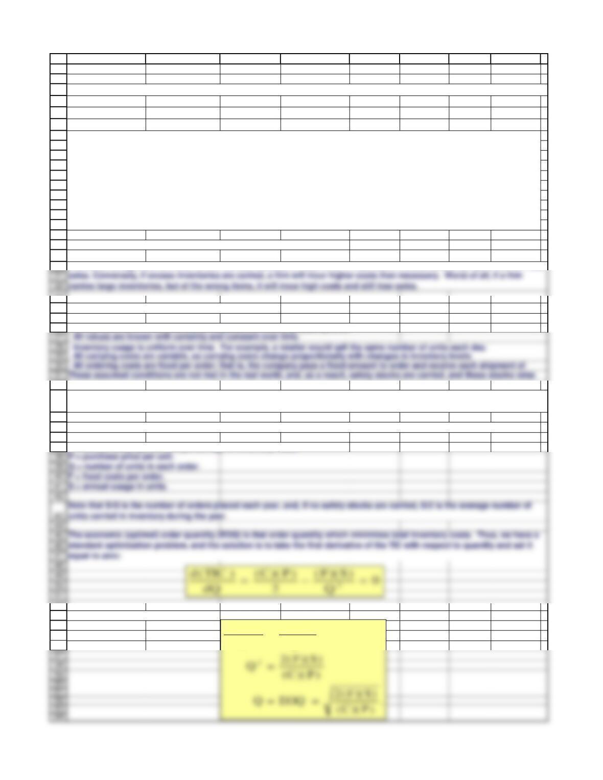
P = purchase price per unit.
Q = number of units in each order.
F = fixed costs per order.
S = annual usage in units.
units carried in inventory during the year.
The economic (optimal) order quantity (EOQ) is that order quantity which minimizes total inventory costs. Thus, we have a
equal to zero:
52
53
54
55
56
57
58
59
60
61
62
63
64
A B C D E F G H I
11/23/2018
C = annual carrying cost as a percentage of inventory value.
Solving for Q gives us:
Chapter 28. Mini Case for Advanced Issues in Cash Management and Inventory Control
Andria Mullins, financial manager of Webster Eelectronics, has been asked by the firm’s CEO, Fred Weygandt, to evaluate
the company’s inventory control techniques and to lead a discussion of the subject with the senior executives. Andria
plans to use as an example one of Webster’s “big ticket” items, a customized computer microchip which the firm uses in
its laptop computer. Each chip costs Webster $200, and in addition it must pay its supplier a $1,000 setup fee on each
order. Further, the minimum order size is 250 units; Webster’s annual usage forecast is 5,000 units; and the annual
carrying cost of this item is estimated to be 20 percent of the average inventory value.
Andria plans to begin her session with the senior executives by reviewing some basic inventory concepts, after which
she will apply the EOQ model to Webster’s microchip inventory. As her assistant, you have been asked to help her by
answering the following questions:
a. Why is inventory management vital to the health of most firms?
b. What assumptions underlie the EOQ Model?
The standard form of the EOQ model requires the following assumptions:
TIC = total carrying costs + total ordering costs = CP(Q/2) + F(S/Q)
Inventory management is critical to the financial success of most firms. If insufficient inventories are carried, a firm will lose
c. Write out the formula for the total costs of carrying and ordering inventory, and then use the formula to derive the EOQ
model.
Q
)S)(F(
2
)P)(C(
2
=
21
22
carries large inventories, but of the wrong items, it will incur high costs and still lose sales.
65
66
67
68
69
70
71
72
84
85
86
87
88
89
90
94
95
96
97
98
99
100
101
then Webster must reorder each time its inventory reaches 2(96) = 192 units. Then, after 2 weeks, as it uses its last
microchip, the new order of 500 chips arrives.
102
103
104
105
106
107
108
109
110
111
112
113
114
115
116
117
could rise to 392/2 = 196 units per week over the 2-week delivery period without causing a stockout. Similarly, if usage
remains at the expected 96 units per week, Webster could operate for 392/96 » 4 weeks versus the normal two weeks while
awaiting delivery of an order.
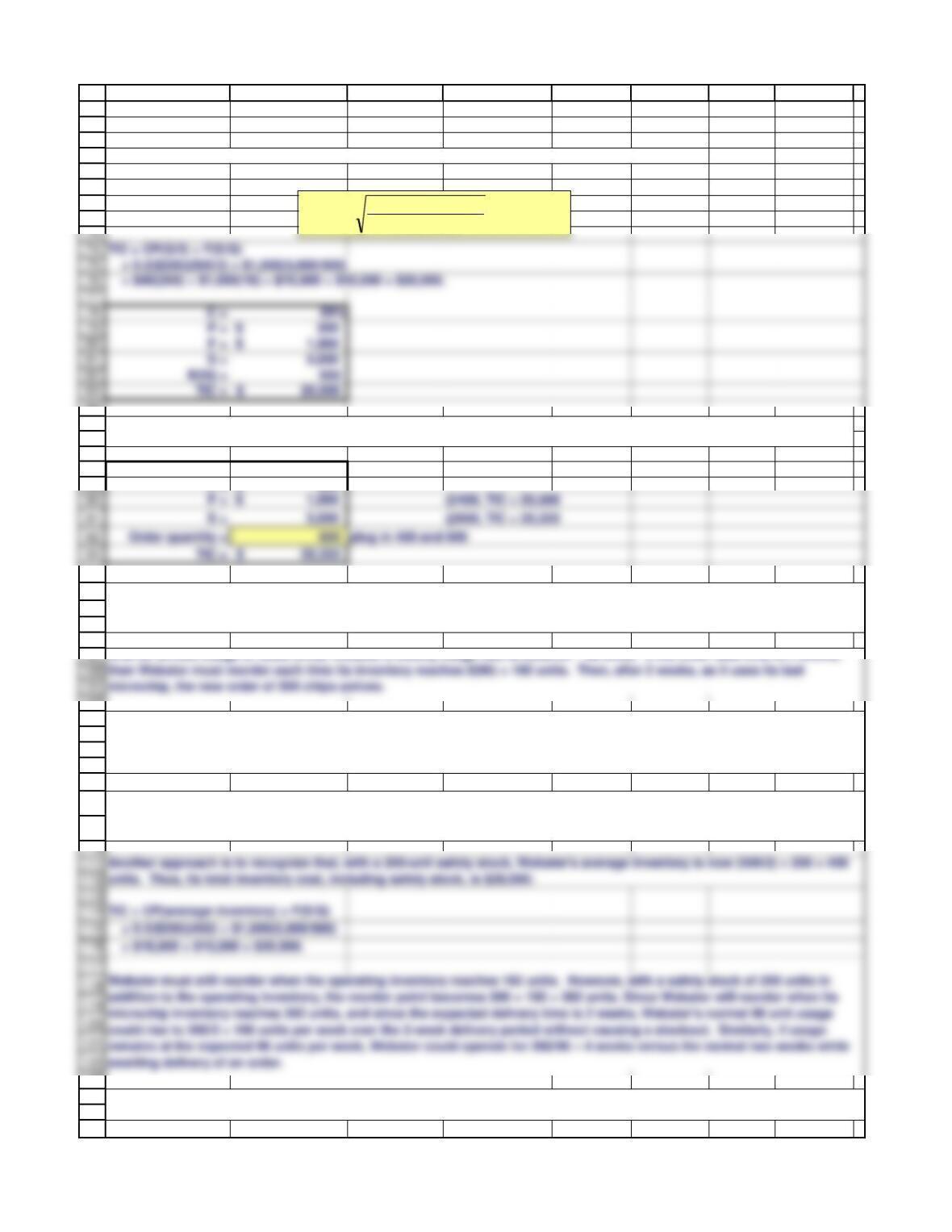
Another approach is to recognize that, with a 200-unit safety stock, Webster’s average inventory is now (500/2) + 200 = 450
units. Thus, its total inventory cost, including safety stock, is $28,000:
123
124
125
126
A B C D E F G H I
C = 20%
P = $ 200
With an annual usage of 5,000 units, Webster’s weekly usage rate is 5,000/52 ~ 96 units. If the order lead time is 2 weeks,
g. Of course, there is uncertainty in Webster’s usage rate as well as in delivery times, so the company must carry a safety
stock to avoid running out of chips and having to halt production. If a 200-unit safety stock is carried, what effect would
this have on total inventory costs? What is the new reorder point? What protection does the safety stock provide if usage
increases, or if delivery is delayed?
d. What is the EOQ for custom microchips? What are total inventory costs if the EOQ is ordered?
f. Suppose it takes 2 weeks for Webster’s supplier to set up production, make and test the chips, and deliver them to
Webster’s plant. Assuming certainty in delivery times and usage, at what inventory level should Webster reorder? (assume
a 52-week year, and assume that Webster orders the EOQ amount.
e. What is Webster’s added cost if it orders 400 units at a time rather than the EOQ quantity? What if it orders 600 per
order?
There are two ways to view the impact of safety stocks on total inventory costs. Webster’s total cost of carrying the
operating inventory is $20,000 (see part d). Now the cost of carrying an additional 200 units is CP(safety stock) =
0.2($200)(200) = $8,000. Thus, total inventory costs are increased by $8,000, for a total of $20,000 + $8,000 = $28,000.
h. Now suppose Webster’s supplier offers a discount of 1 percent on orders of 1,000 or more. Should Webster take the
discount? Why or why not?
units500
)200($2.0
)000,5)(000,1($2
EOQ ==
73
74
75
76
77
78
79
80
81
82
83
C = 20%
P = $ 200
S = 5,000
127
128
129
130
131
135
136
137
138
139
140
141
142
143
144
145
146
147
148
149
150
151
152
153
154
155
156
157
158
159
160
161
(2.) The use of air freight for deliveries.
Air freight would presumably shorten delivery times and reduce the need for safety stocks. It might or might not affect the
Just-in-time procedures are designed specifically to reduce inventories. If a just in time system were put in place, it would
largely obviate the need for using the EOQ model.
(1.) The use of just-in-time procedures.
162
163
164
165
166
167
168
Computerized control systems would, generally, enable the company to keep better track of its existing inventory. This
would probably reduce safety stocks, and it might or might not affect the EOQ.
169
170
171
172
173
174
176
177
This reduces inventory holdings of final goods.
178
179
180
181
182
183
184
185
186
187
188
189
Total cash needs per year 1,200,000.00
EOQ = Optimal cash transfer 33,123
Number of times to liquidate per year 36.2
Number of weeks between liquidations 1.435
A B C D E F G H I
Monthly cash deficit (cash needs) 100,000.00
Opportunity cost for cash 7%
Brokerage costs for each transaction 32
(4.) The manufacturing plant is redesigned and automated. Computerized process equipment and state-of-the-art
robotics are installed, making the plant highly flexible in the sense that the company can switch from the production of
one item to another at a minimum cost and quite quickly. This makes short production runs more feasible than under the
old plant setup.
(3.) The use of a computerized inventory control system, wherein as units were removed from stock, an electronic
system automatically reduced the inventory account and, when the order point was hit, automatically sent an electronic
message to the supplier placing an order. The electronic system ensures that inventory records are accurate, and that
orders are placed promptly.
Applying this to cash management:
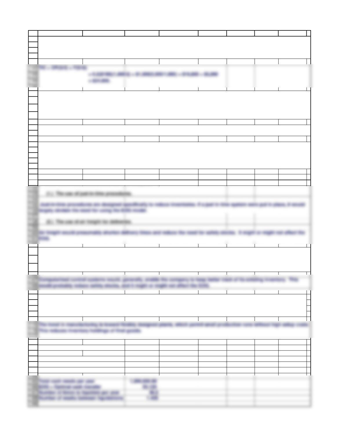
Note that we have reduced the unit price by the amount of the discount. Since total costs are $24,800 if Webster orders
1,000 chips at a time, the incremental annual cost of taking the discount is $24,800 – $20,000 = $4,800. However, Webster
would save 1 percent on each chip, for a total annual savings of 0.01($200)(5,000) = $10,000. Thus, the net effect is that
Webster would save $10,000 – $4,800 = $5,200 if it takes the discount, and hence it should do so.
First, note that since the discount will only affect the orders for the operating inventory, the discount decision need not take
account of the safety stock. Webster’s current total cost of its operating inventory is $20,000 (see part d). If Webster
increases its order quantity to 1,000 units, then its total costs for the operating inventory would be $24,800:
i. For many firms, inventory usage is not uniform throughout the year, but, rather, follows some seasonal pattern. Can the
EOQ model be used in this situation? If so, how?
The EOQ model can still be used if there are seasonal variations in usage, but it must be applied to shorter periods during
which usage is approximately constant. For example, assume that the usage rate is constant, but different, during the
summer and winter periods. The EOQ model could be applied separately, using the appropriate annual usage rate, to each
period, and during the transitional fall and spring seasons inventories would be either run down or built up with special
seasonal orders.
j. How would these factors affect an EOQ analysis?
132
133
134
190
191
192
193
A B C D E F G H I
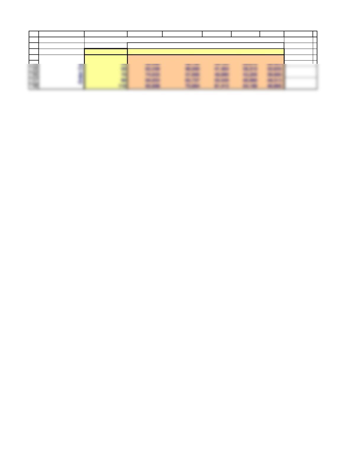
33,123 3% 5% 7% 9% 11%
10 28,284 21,909 18,516 16,330 14,771
Carrying Cost
Optimal cash transfer size for various order costs and carrying costs
194
195
196
197
198
32 50,596 39,192 33,123 29,212 26,423
50 63,246 48,990 41,404 36,515 33,029
70 74,833 57,966 48,990 43,205 39,080
90 84,853 65,727 55,549 48,990 44,313