
11/23/2018
REAL OPTIONS: THE INVESTMENT TIMING OPTION
Chapter 26. Real Options
a. What are some types of real options? Answer: See Chapter 26 Mini Case Show
b. What are the five steps for analyzing a real option? Answer: See Chapter 26 Mini Case Show
c. Tropical Sweets is considering a project that will cost $70 million and will generate expected cash flows of
$30 per year for three years. The cost of capital for this type of project is 10 percent and the risk-free rate is 6
percent. After discussions with the marketing department, you learn that there is a 30 percent chance of high
demand, with future cash flows of $45 million per year. There is a 40 percent chance of average demand, with
cash flows of $30 million per year. If demand is low (a 30 percent chance), cash flows will be only $15 per year.
What is the expected NPV?
could use to gain at least a cursory understanding of the topics.
Assume that you have just been hired as a financial analyst by Tropical Sweets Inc., a mid-sized California
company that specializes in creating exotic candies from tropical fruits such as mangoes, papayas, and dates.
The firm’s CEO, George Yamaguchi, recently returned from an industry corporate executive conference in San
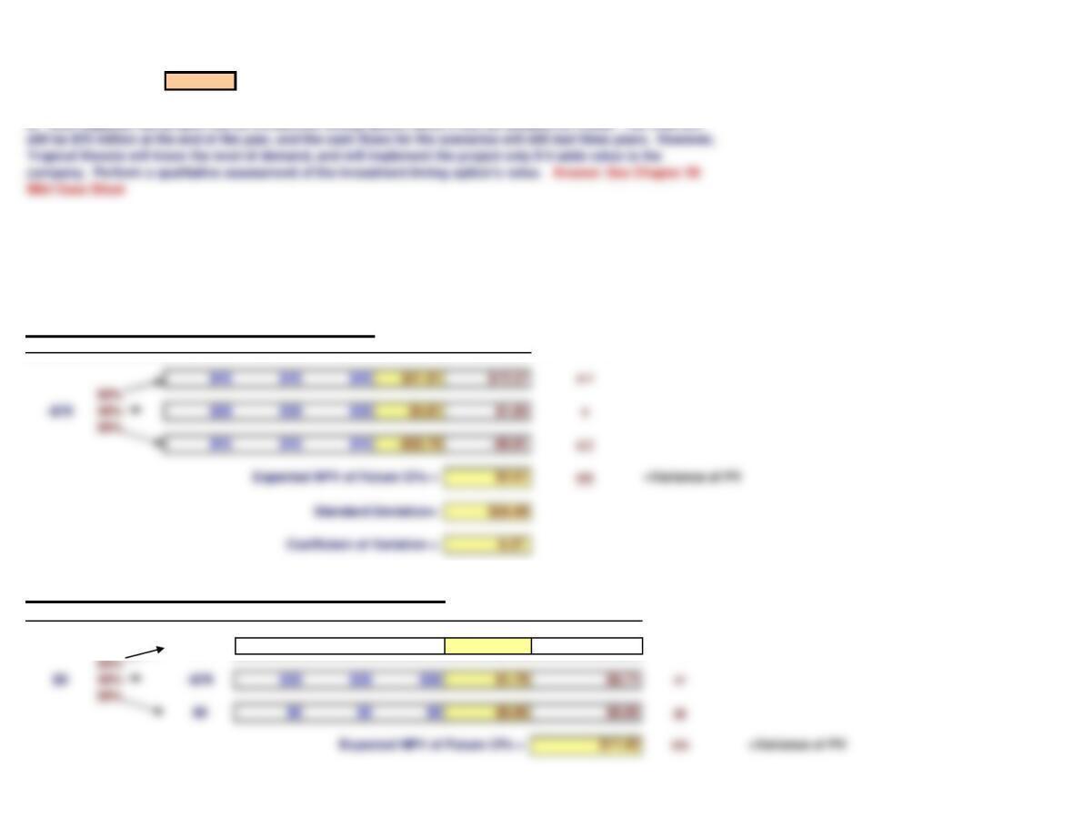
NPV= $4.61
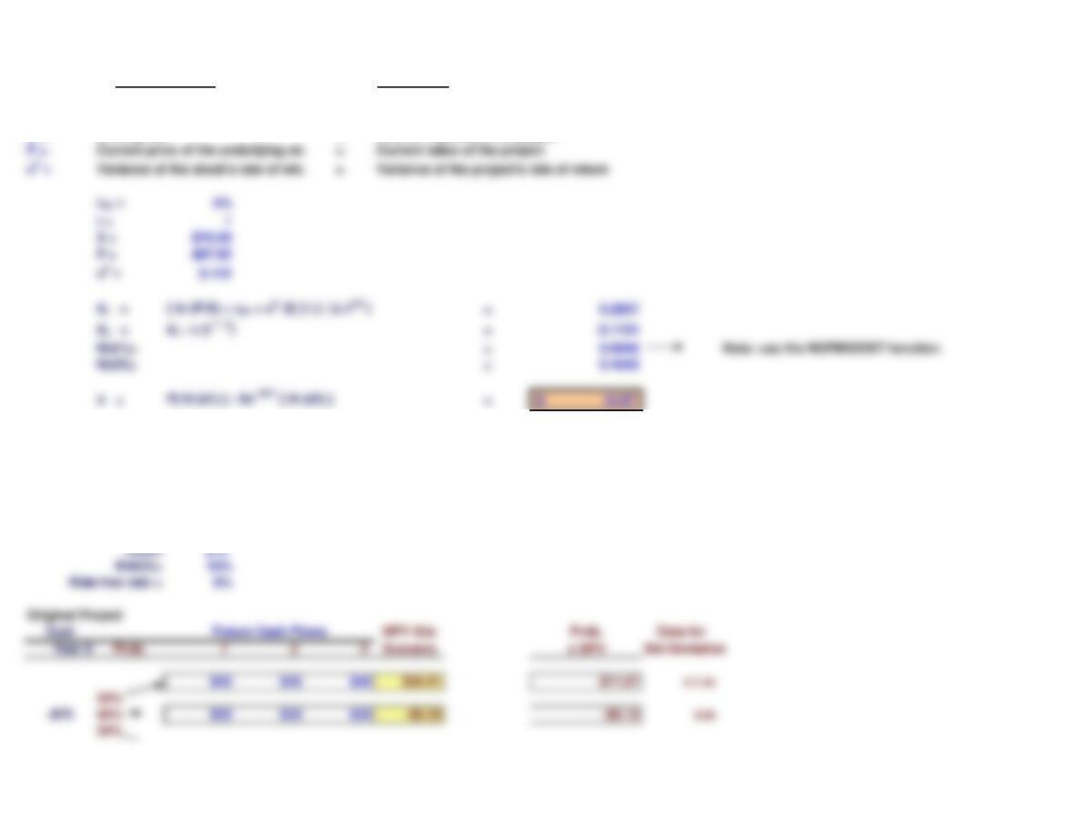
Procedure 3: Decision Tree Analysis
a. Scenario Analysis: Proceed with Project Today
Cost NPV this Prob. Data for
Year 0 Prob. 1 2 3 Scenario x NPV
b. Decision Tree Analysis: Implement in One Year Only if Optimal
Cost NPV this Prob. Data for
Year 0 Prob. 12 3 4
Scenarioax NPV
-$70 $45 $45 $45 $35.70 $10.71 177
Future Cash Flows
Future Cash Flows
Std Deviation
Std Deviation
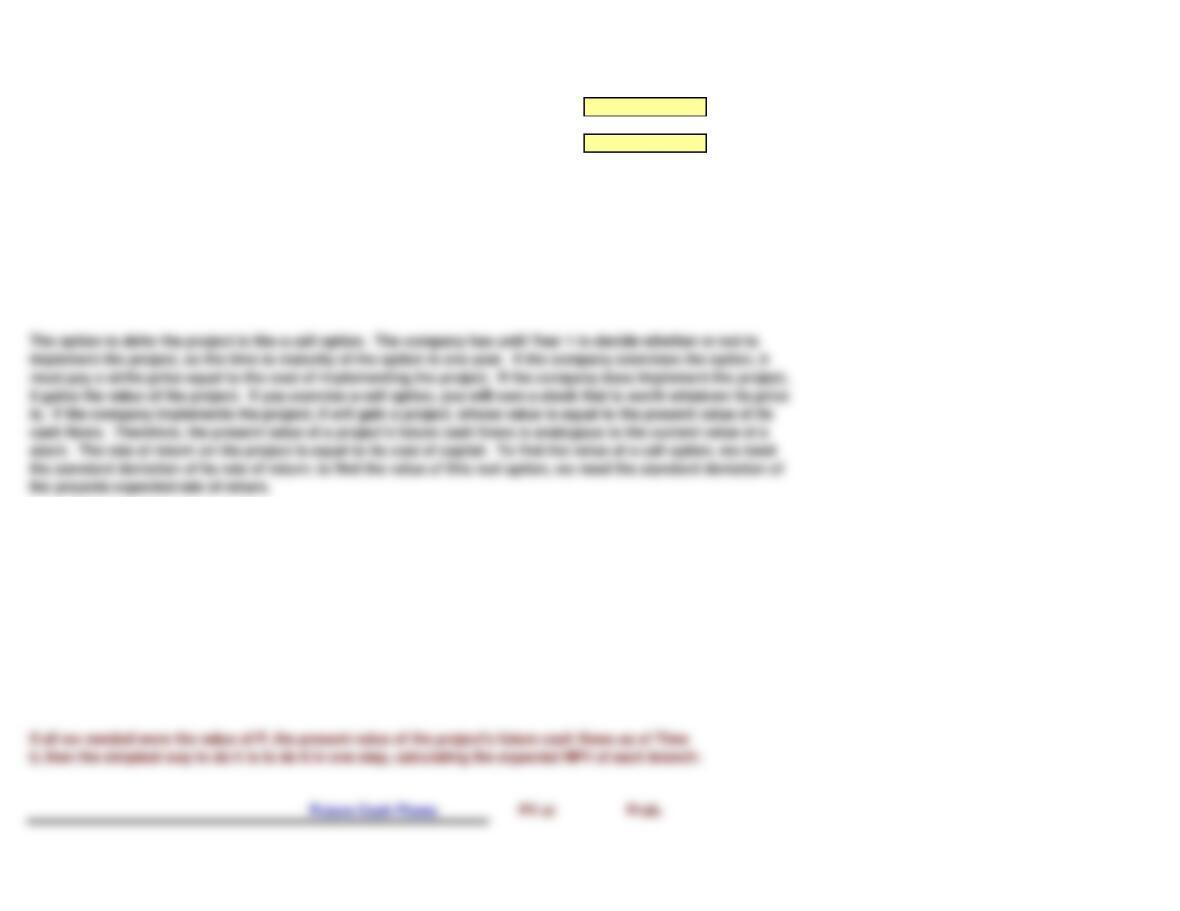
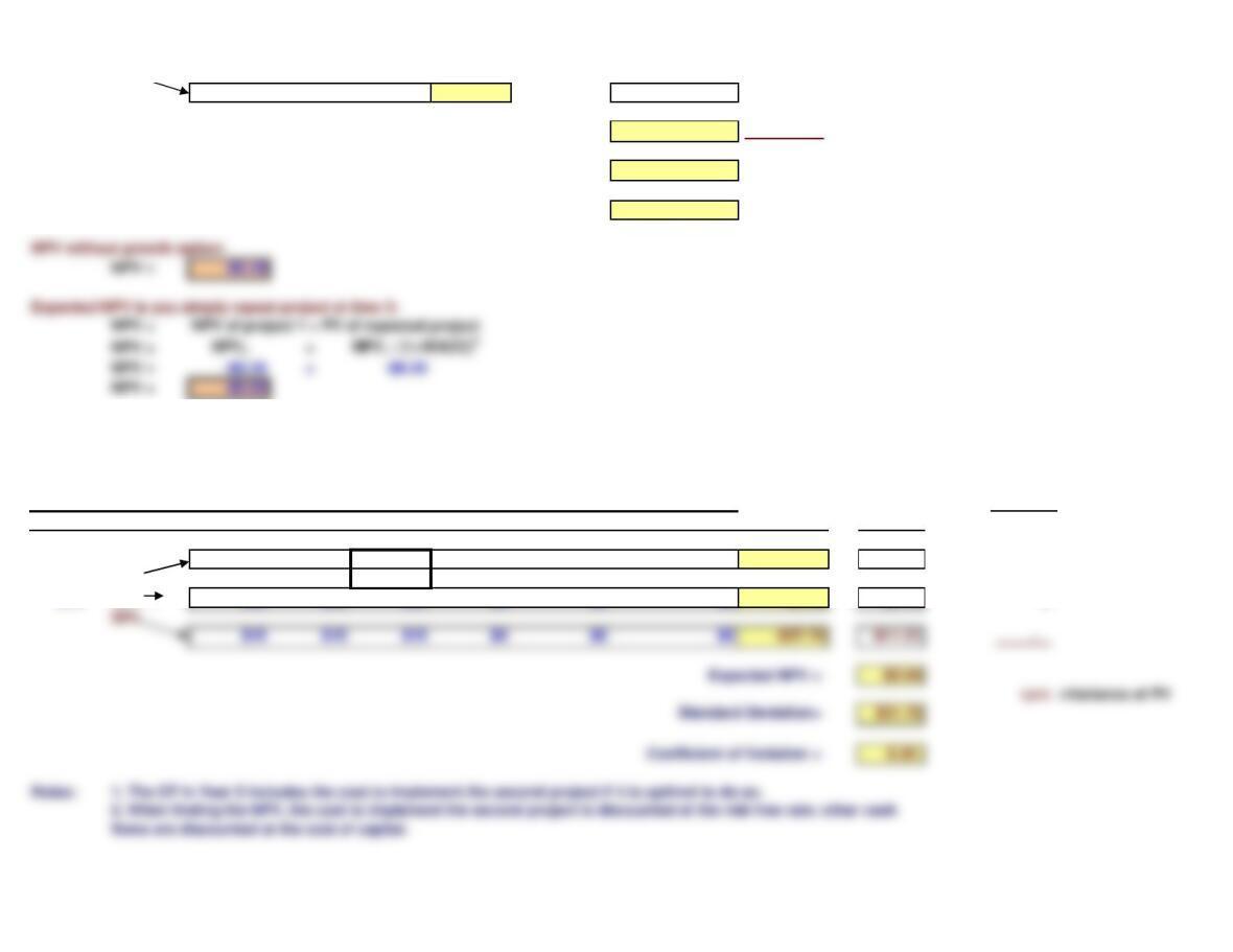
d. Now suppose this project has an investment timing option, since it can be delayed for a year. The cost will
e. Use decision tree analysis to calculate the NPV of the project with the investment timing option.
Standard Deviation= $15.91
Coefficient of Variation = 1.39
Notes:
Procedure 4: Analysis with a Financial Option
Find the Year 0 Value of Future Cash Flows
a Discount the cost of the project at the risk-free rate, since the cost is known. Discount
the operating cash flows at the WACC.
Thus we need to calculate two values from the tree of the project’s outcomes in order to implement the Black
Scholes Option Pricing Model. We need P, which is the present value of the project’s future cash flows as of
Time 0. We also need the standard deviation, s, of the project’s return as of the date it must be exercised. We will
find P in two different ways. The first is the most intuitive and we show it to help you better understand what is
going on. The second takes an extra step but is useful because it generates information we can use in
calculating the standard deviation of return.
f. Use a financial option pricing model to estimate the value of the investment timing option.
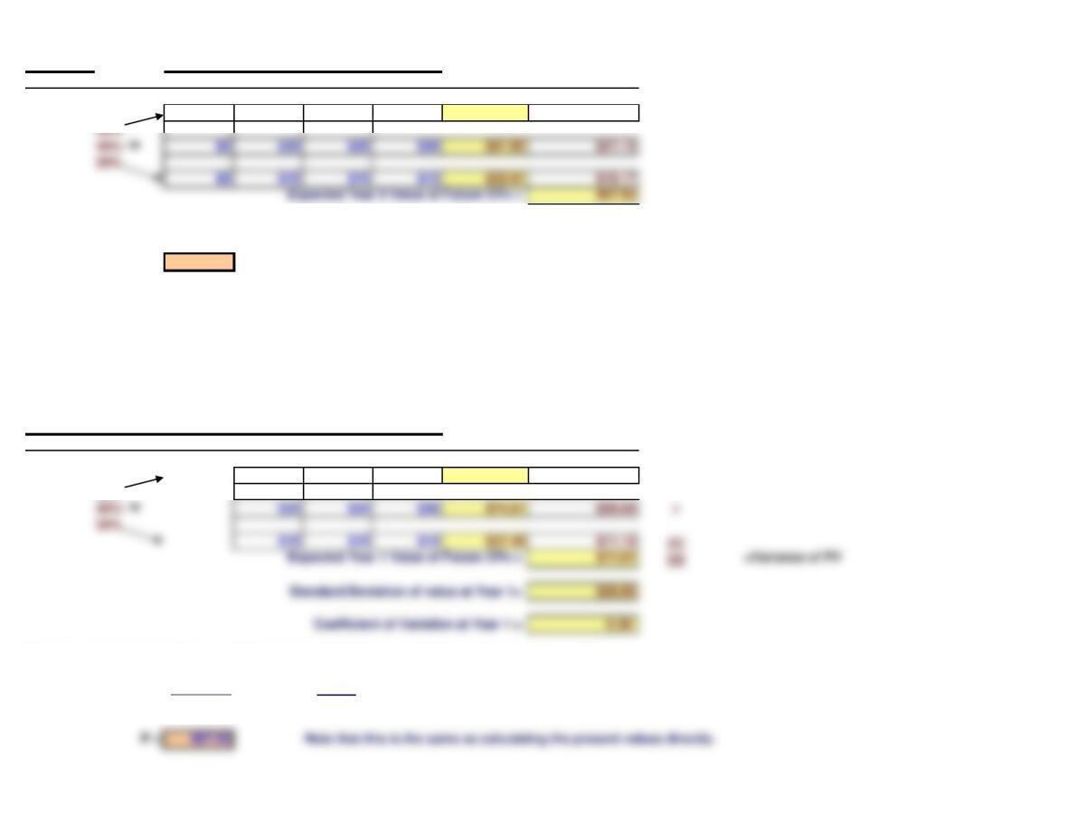
Year 0 Prob. 1 2 3 4 Year 0 x Value
$0 $45 $45 $45 $101.73 $30.52
P is the expected present value (as of Time 0) of the project’s future cash flows.
P = $67.82
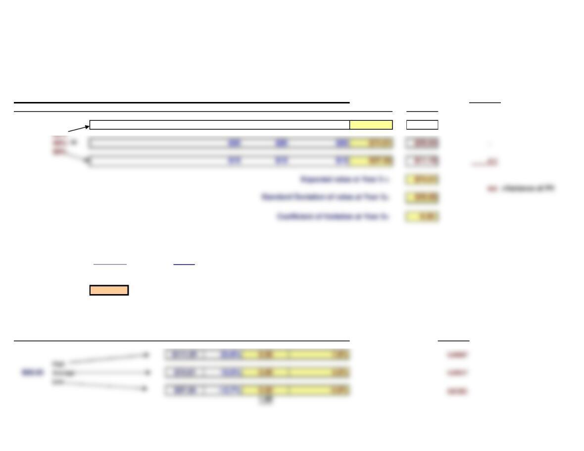
Find the Year 1 Value and Risk of Future Cash Flows If Project is Deferred
PV at Prob. Data for
Year 0 Prob. 1 2 3 4 Year 1 x Value
$45 $45 $45 $111.91 $33.57 417
30%
30%
Find the current value of future cash flows if project is deferred (note: this is the estimate of P).
Current Value = Year 1 Value =$74.61 =$67.82
(1+WACC) 1.10
P = $67.82 Note that this is the same as calculating the present values directly.
However, since we will also need some information about the value of the cash flows at Time 1 to
use in the standard deviation, we will in later examples use this second method. We start by
calculating the present value of the project’s future cash flows as of Time 1.
Std Deviation
Future Cash Flows
30%
30%
$0 $15 $15 $15 $33.91 $10.17
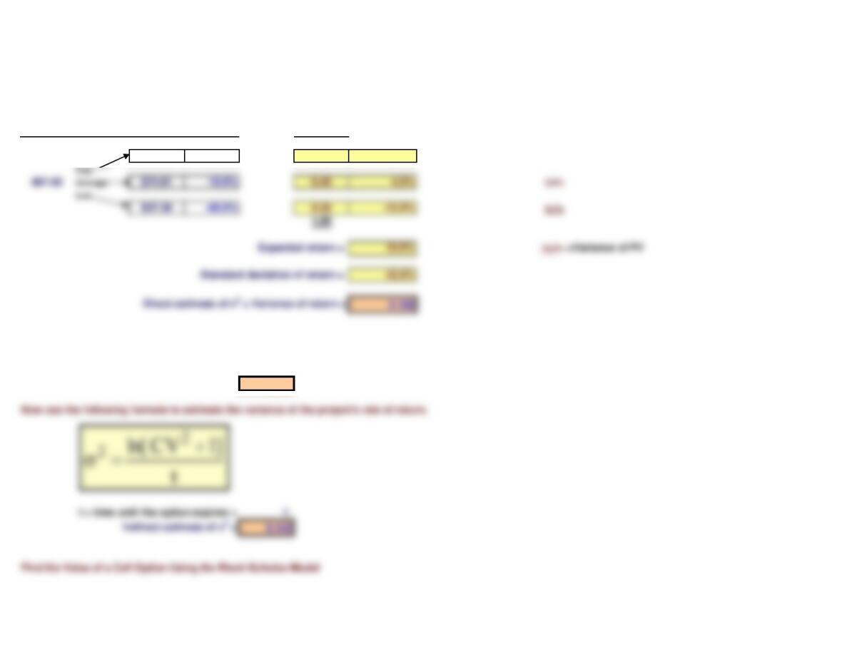
Use the direct approach to estimate the variance of the project‘s rate of return.
Probability Data for
PVYear 0 PVYear 1 Return Probability
$111.91 65.00% 0.30 19.5% 9.1%
CV =Coefficient of Variation = 0.39
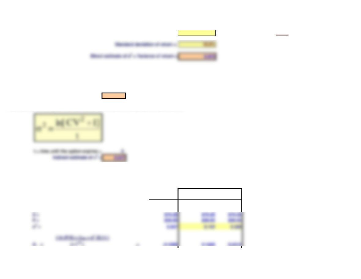
Now use the following formula to estimate the variance of the project’s rate of return.
Find the Value of a Call Option Using the Black-Scholes Model
Std Deviation
Use the indirect approach to estimate the variance of the project’s rate of return. Start by estimating the coefficient of
variation, CV, of the project‘s value at the time the option expires. This was done in an earlier step.
x ReturnYear 1
Real Option
rRF = Risk-free interest rate = Risk-free interest rate
t = Time until the option expires = Time until the option expires
X = Strike price = Cost to implement the project
REAL OPTIONS: THE GROWTH OPTION
g. Now suppose the cost of the project is $75 million and the project cannot be delayed. But if Tropical Sweets
implements the project, then Tropical Sweets will have a growth option. It will have the opportunity to replicate the
original project at the end of its life. What is total expected NPV of the two projects if both are implemented?
Financial Option
P =
$15 $15 $15 -$37.70 -$11.31 417.45
Expected NPV = -$0.39 834.90 =Variance of PV
Standard Deviation= $28.89
Coefficient of Variation = (73.25)
Decision Tree: Implement the repeated project only if demand is high. Data for
Cost NPV this Prob. Std Deviation
Year 0 Prob. 1 2 3 4 5 6 Scenario x NPV
$45 $45 $45 $45 $45 $45 $58.02 $17.40 1,010
30% -$75
-$75 40% $30 $30 $30 $0 $0 $0 –$0.39 -$0.16 0
2. When finding the NPV, the cost to implement the second project is discounted at the risk-free rate; other cash
flows are discounted at the cost of capital.
Future Cash Flows
h. Tropical Sweets will replicate the original project only if demand is high. Using decision tree analysis,
estimate the value of the project with the growth option.
Expected NPV is you simply repeat project at time 3:
Financial Option Approach
Find the value and risk of the future cash flows as of the time the option expires.
Data for
Cost PV at Prob. Std Deviation
Year 0 Prob. 1 2 3 4 5 6 Year 3 x NPV
$45 $45 $45 $111.91 $33.57 417
Find the current value of future cash flows if project is deferred (note: this is the estimate of P).
Current Value = Year 3 Value =$74.61 =$56.05
(1+WACC)3
1.33
P = $56.05
Use the direct approach to estimate the variance of the project‘s rate of return.
Annual Data for
PVYear 0 1 2 PVYear 3 Return Probability x Returnannual Std Deviation
i. Use a financial option model to estimate the value of the growth option.
Future Cash Flows
Expected return = 7.968% 0.02264 =Variance of PV
CV =Coefficient of Variation = 0.39
Now use the following formula to estimate the variance of the project’s rate of return.
Find the Value of a Call Option Using the Black-Scholes Model
Sensitivity Analysis
Base Case Case 1 Case 2
rRF = 6% 6% 6%
t = 3 3 3
X = $75.00 $75.00 $75.00
P = $56.05 $56.05 $56.05
j. What happens to the value of the growth option if the variance of the project’s return is 14.2 percent? What if
it is 50 percent? How might this explain the high valuations of many dot.com companies?
Use the indirect approach to estimate the variance of the project’s rate of return. Start by estimating the coefficient of
variation, CV, of the project‘s value at the time the option expires. This was done in an earlier step.

d2 = d1 – s (t 1 / 2)=-0.4840 -0.4968 -0.7032
N(d1)= = 0.4568 0.5619 0.6990 Note: we used the NORMSDIST function.
N(d2)= = 0.3142 0.3097 0.2410