Chapter 26
Real Options
ANSWERS TO END-OF-CHAPTER QUESTIONS
26-1 a. Real options occur when managers can influence the size and risk of a project’s cash
flows by taking different actions during the project’s life. They are referred to as real
options because they deal with real as opposed to financial assets. They are also called
managerial options because they give opportunities to managers to respond to changing
market conditions. Sometimes they are called strategic options because they often deal
with strategic issues. Finally, they are also called embedded options because they are
a part of another project.
c. Decision trees are a form of scenario analysis in which different actions are taken in
different scenarios.
26-2 Postponing the project means that cash flows come later rather than sooner; however,
waiting may allow you to take advantage of changing conditions. It might make sense,
however, to proceed today if there are important advantages to being the first competitor
to enter a market.
SOLUTIONS TO END-OF-CHAPTER PROBLEMS
Note: We report rounded values, but there is no rounding in intermediate
calculations
26-1 a. 0 1 2 20
├─────┼─────┼────── • • • ────┤
-20 3 3 3
NPV = $1.074 million.
b. Wait 1 year:
PV @
Answers and Solutions: 26 – 3
26-2 a. 0 1 2 3 4
├─────┼─────┼─────┼─────┤
-8 4 4 4 4
NPV = $4.68 million.
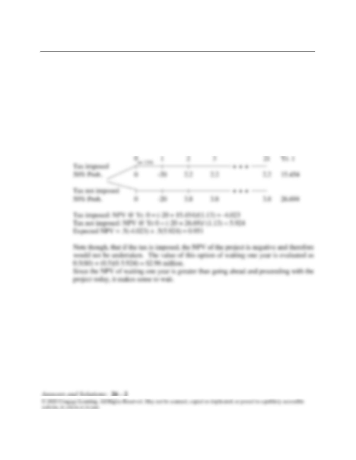
b. Wait 2 years:
If the cash flows are only $2.2 million, the NPV of the project is negative and, thus,
would not be undertaken. The value of the option of waiting two years is evaluated as
0.10($0) + 0.90($3.56) = $3.21 million.
Since the NPV of waiting two years is less than going ahead and proceeding with the
project today, it makes sense to drill today.
10%
Answers and Solutions: 26 – 4
b. Option to sell:
If Wansley sells the company at Year 2 it will forego 18 years of cash flows and receive
$280 million instead. The NPV of 18 years of $50 million per year at a 13% discount rate
is $342 million, so Wansley would not sell the company at Year 2 if the good cash flows
happened.
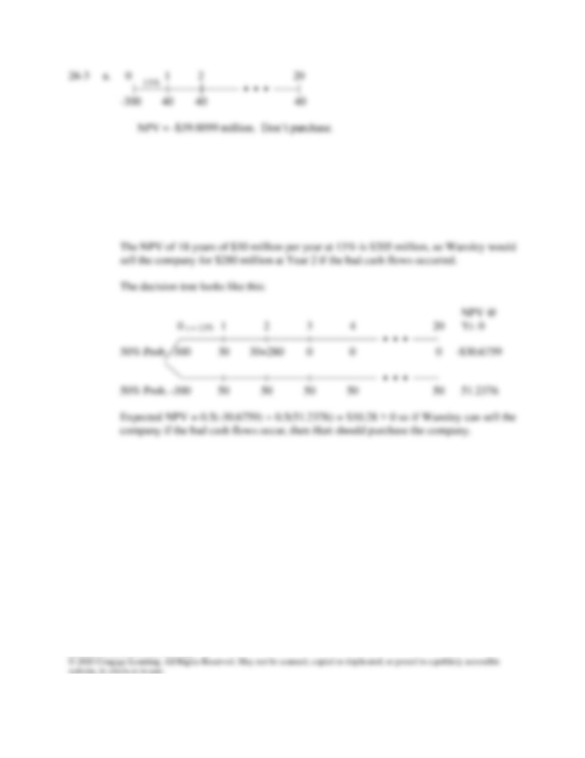
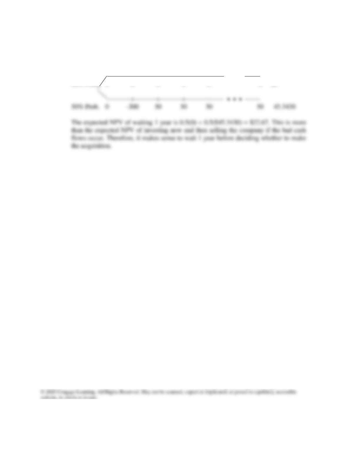
c. Wait 1 year:
If Wansley waits to purchase the company, it can’t later sell it for $280 million.
If the bad cash flows occur, then the NPV of the investment as of Year 1 is -$89.26 = the
NPV of –300, 30, 30, ….30, so Wansley would choose not to invest if the bad cash flows
occur.
Answers and Solutions: 26 – 5
So the decision tree would then look like this:
NPV @
0 1 2 3 4 21 Yr. 0
| | | | | • • • |
50% Prob. 0 0 0 0 0 0 $0
r = 13%
Answers and Solutions: 26 – 6
26-4 a. 0 1 14 15
b. 0 1 14 15
| | • • • | |
−6,200,000 1,200,000 1,200,000 1,200,000
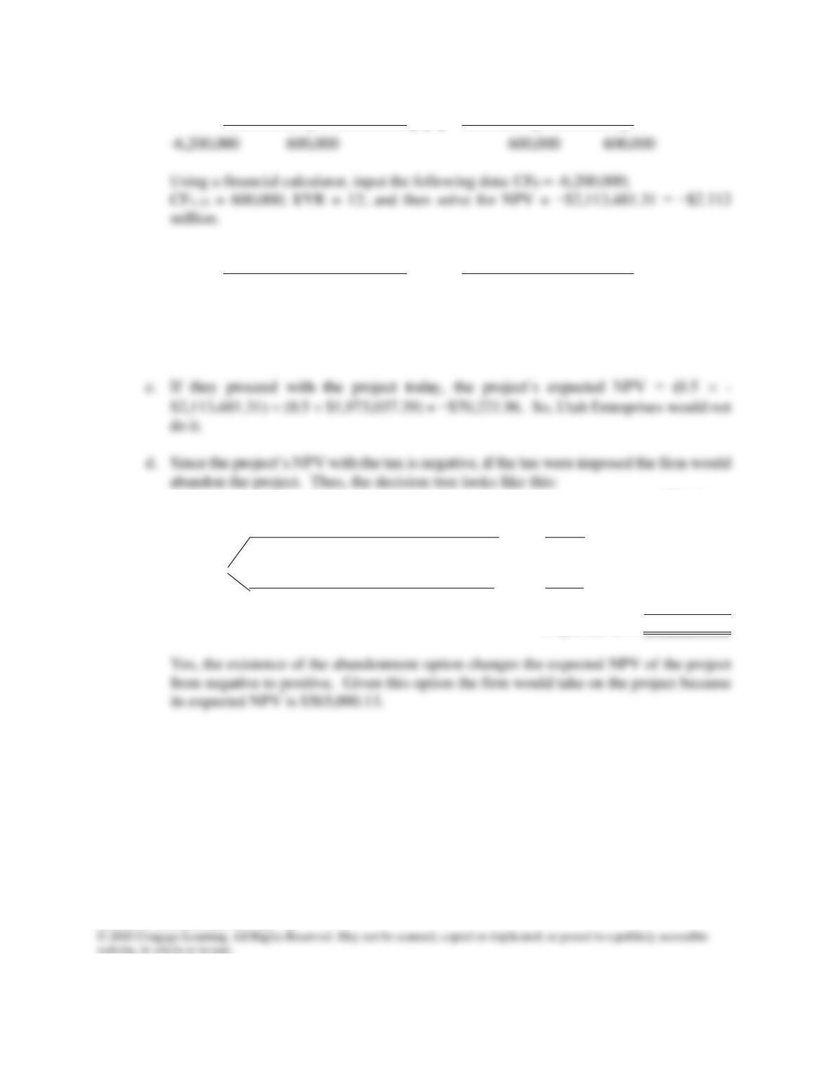
Using a financial calculator, input the following data: CF0 = -6,200,000;
CF1-15 = 1,200,000; I/YR = 12; and then solve for NPV = $1,973,037.39 = $1.973 million.
NPV @
0 1 2 15 Yr. 0
50% Prob. | | | • • • |
Taxes -6,200,000 6,000,000 0 0 -$ 842,857.14
No Taxes | | | • • • |
50% Prob. -6,200,000 1,200,000 1,200,000 1,200,000 1,973,037.39
Expected NPV $ 565,090.13
12%
12%
r= 12%
Answers and Solutions: 26 – 7
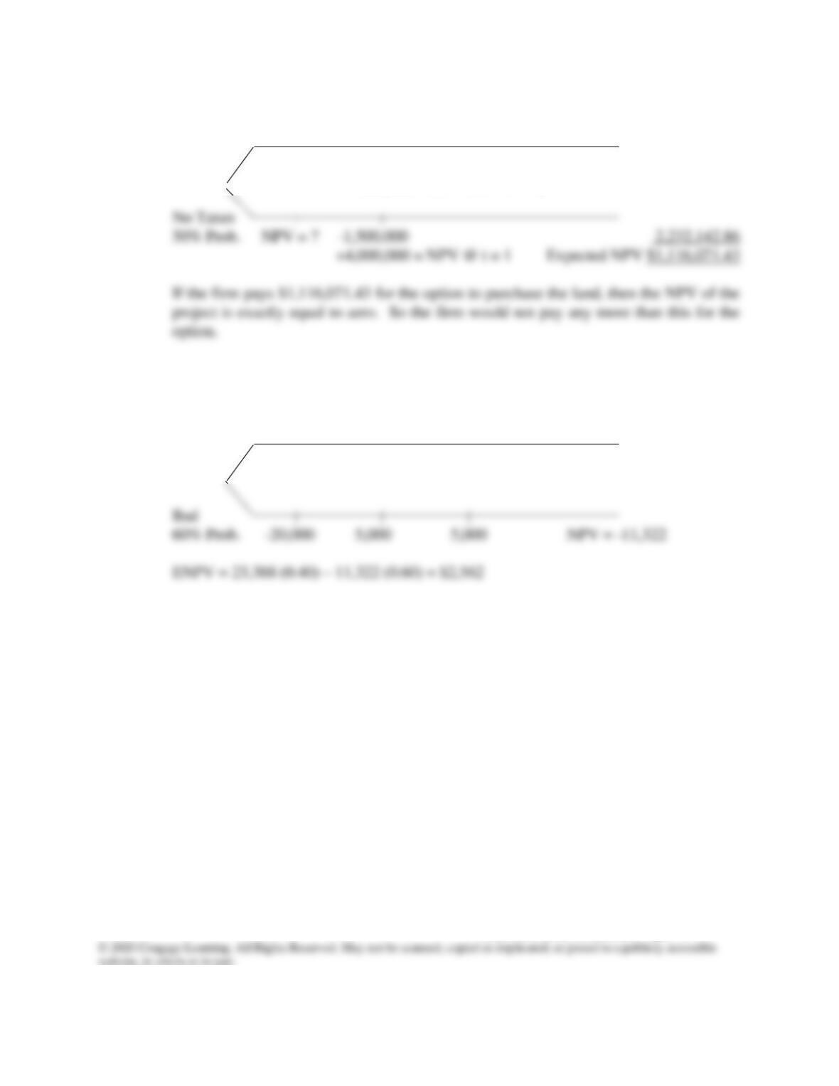
e. NPV @
0 1 Yr. 0
50% Prob. | |
Taxes NPV = ? -1,500,000 $ 0.00
+300,000 = NPV @ t = 1
26-5
a.
0 1 2
40% Prob. | | |
Good –20,000 25,000 25,000 NPV = 23,388
r = 12%
wouldn’t do
r = 10%
Answers and Solutions: 26 – 8
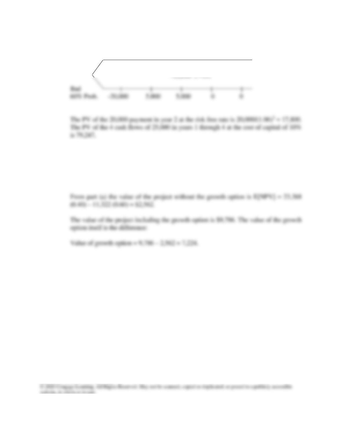
b.
0 1 2 3 4
40% Prob. | | | | |
Good –20,000 25,000 25,000 25,000 25,000
The NPV of the top row is 79,247 – 20,000 – 17,800 = 41,447.
The NPV of the bottom row is still -11,332, as it was in part a.
The expected NPV, E[NPV], is 41,447 (0.40) –11,332 (0.60) = $9,786.
r = 10%
26-6 P = PV of all expected future cash flows if project is delayed. From Problem 26-1 we
know that PV @ Year 1 of Tax Imposed scenario is $15.45 and PV @ Year 1 of Tax Not
Imposed Scenario is $26.69. So the expected PV at Year 0 is:
P = [0.5(15.45)+ 0.5(26.690] / 1.13 = $18.650.
From Excel function NORMSDIST, or approximated from the table in Appendix A:
N(d1) = 0.5673
N(d2) = 0.4631
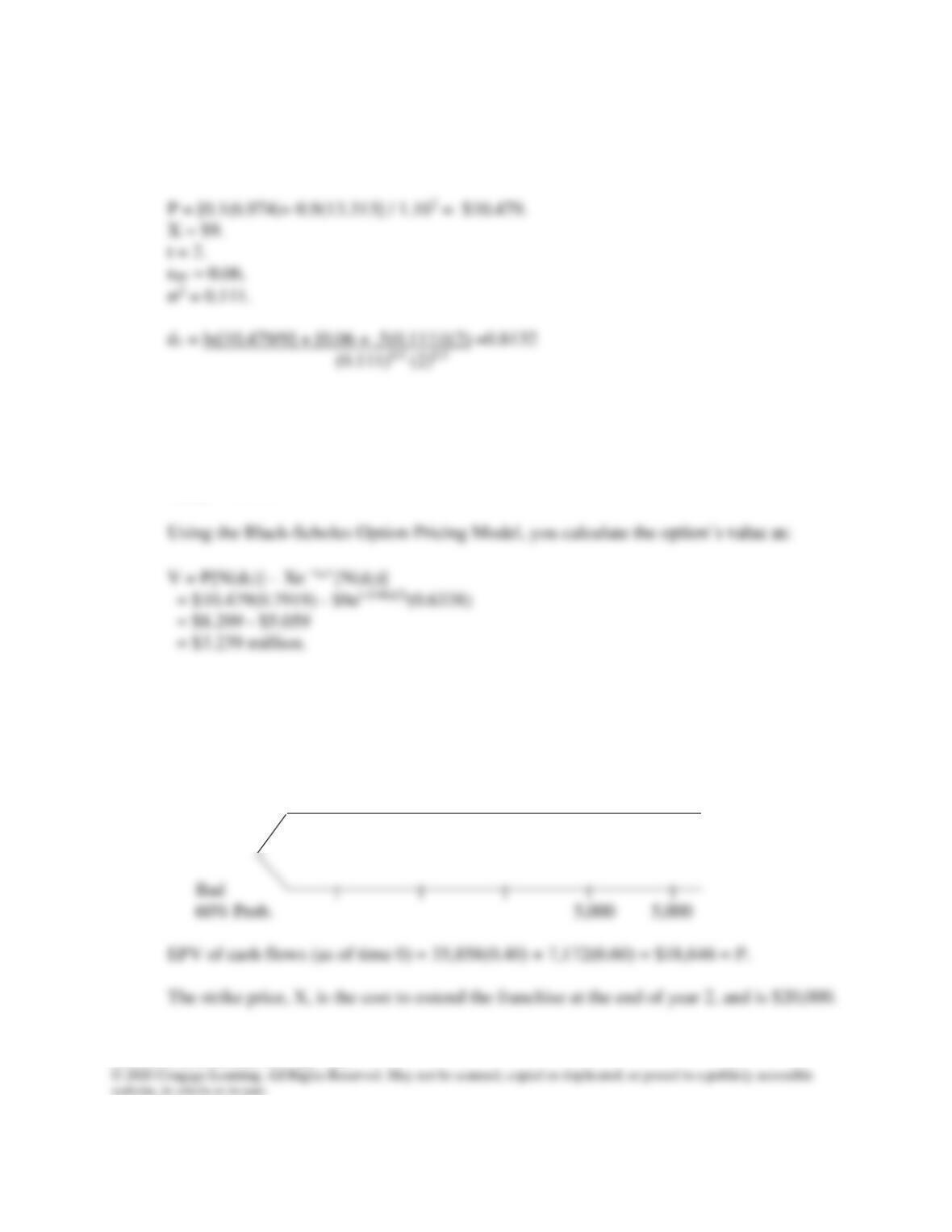
Using the Black-Scholes Option Pricing Model, you calculate the option’s value as:
Answers and Solutions: 26 – 10
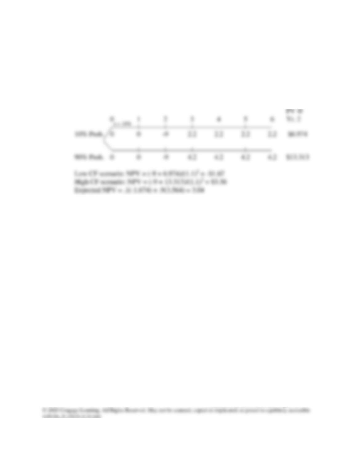
26-7 P = PV of all expected future cash flows if project is delayed. From Problem 26-1 we
know that PV @ Year 2 of Low CF Scenario is $6.974 and PV @ Year 2 of High CF
Scenario is $13.313. So the PV is:
d2 = 0.8132 – (0.111)0.5 (2)0.5 = 0.3420
From Excel function NORMSDIST, or approximated from the table in Appendix A:
N(d1) = 0.7919
N(d2) = 0.6338
26-8 P = PV as of time zero of all expected future cash flows if the project is repeated starting
in year 2. Note it includes both the good cash flows and the bad cash flows since as of
now, we don’t know which outcome will result, and P excludes the $20,000 investment in
the franchise.
0 1 2 3 4
40% Prob. | | | | |
Good 25,000 25,000
r = 10%
Answers and Solutions: 26 – 11
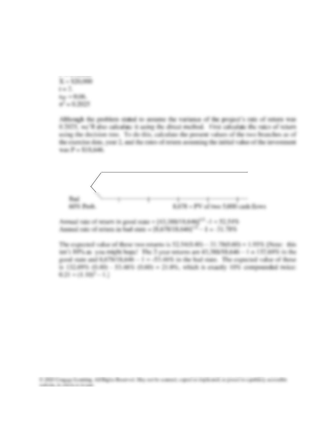
The time to expiration is the time you decide whether or not to extend the franchise, and is
at the end of year 2.
0 1 2 3 4
40% Prob. | | | | |
Good 43,388 = PV of two 25,000 cash flows
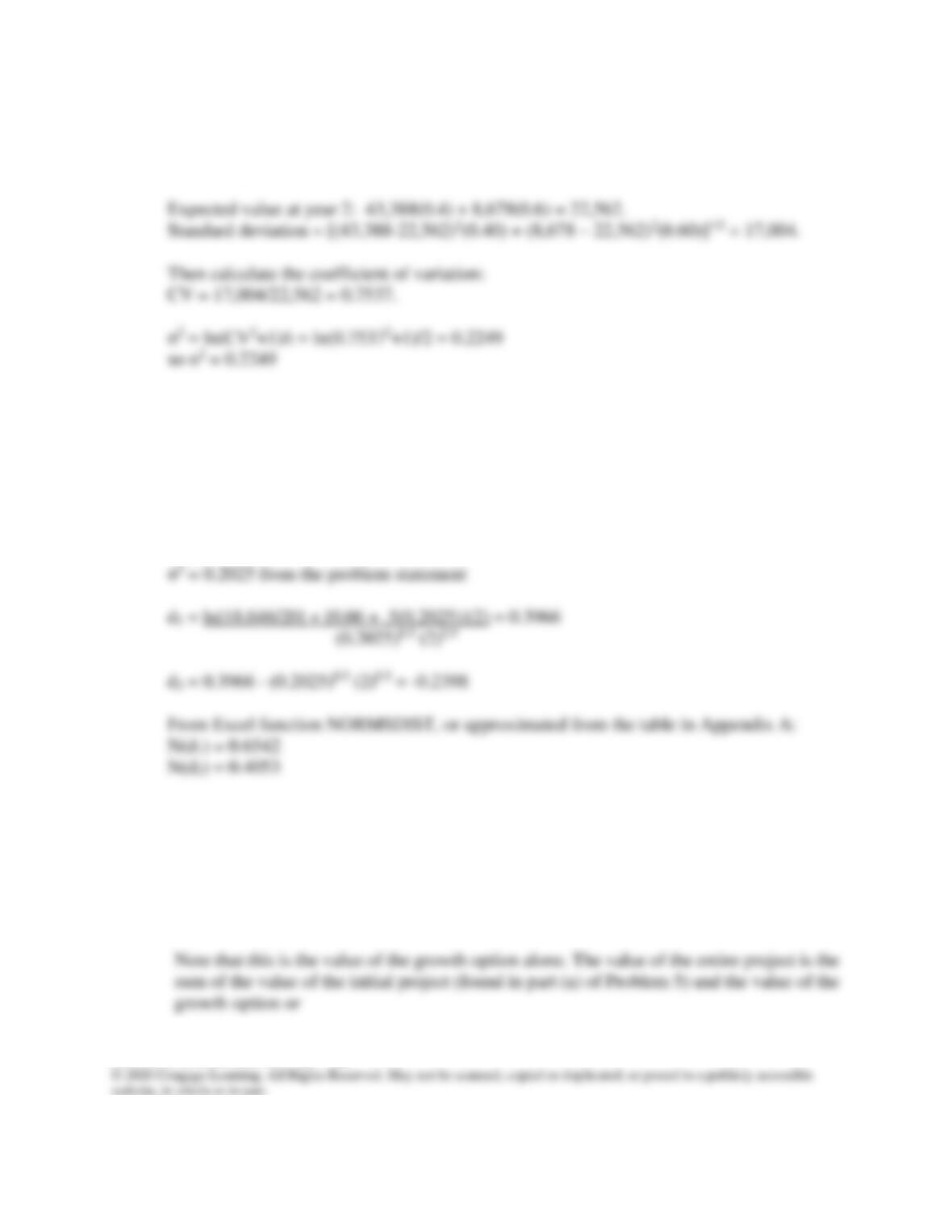
The variance is
σ2 = (0.5254 – 0.0195)2(0.40) + (-0.3178 – 0.0195)2 (0.60) = 0.1706
Answers and Solutions: 26 – 12
To calculate the variance of the project’s returns using the indirect method, first calculate
the standard deviation of the value at year 2. The value is either 43,388 (probability 40%)
or 8,678 (probability 60%).
Notice that in this case the direct method and the indirect method give very similar results
for σ.
Using the assumed variance from the problem statement:
P = $18,646
X = $20,000
t = 2.
rRF = 0.06.
Using the Black-Scholes Option Pricing Model, you calculate the option’s value as:
V = P[N(d1)] –
trRF
Xe −
[N(d2)]
= $18.646(0.6542) – $20e(-0.06)(2)(0.4053)
= $12.198 – $7.189
= $5.009 thousand.


Answers and Solutions: 26 – 14
SOLUTION TO SPREADSHEET PROBLEMS
26-9 The detailed solution for the problem is available in the file, Ch 26 P9 Build a Model
Solution.xlsx, on the textbook’s Web site.