Mini Case: 25 – 12
20%
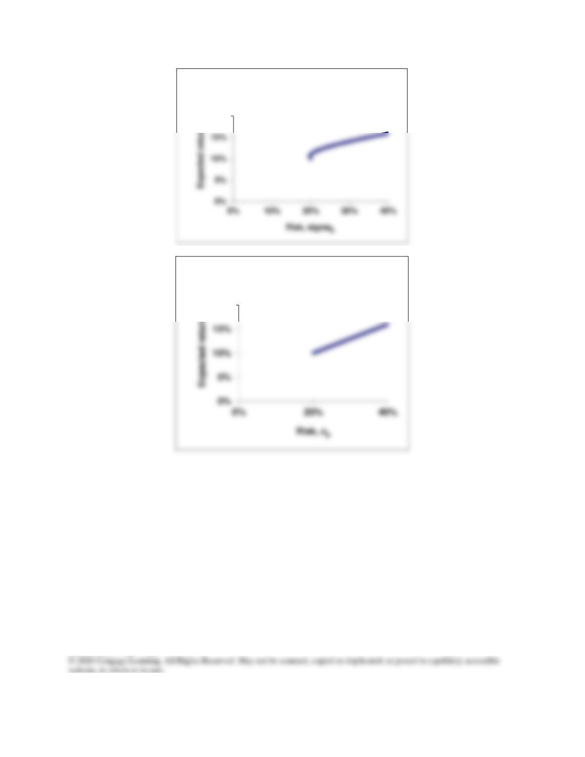
pAB = +0.35: Attainable Set of
Risk/Return Combinations
20%
AB = +1.0: Attainable Set of Risk/Return
Combinations
Mini Case: 25 – 13
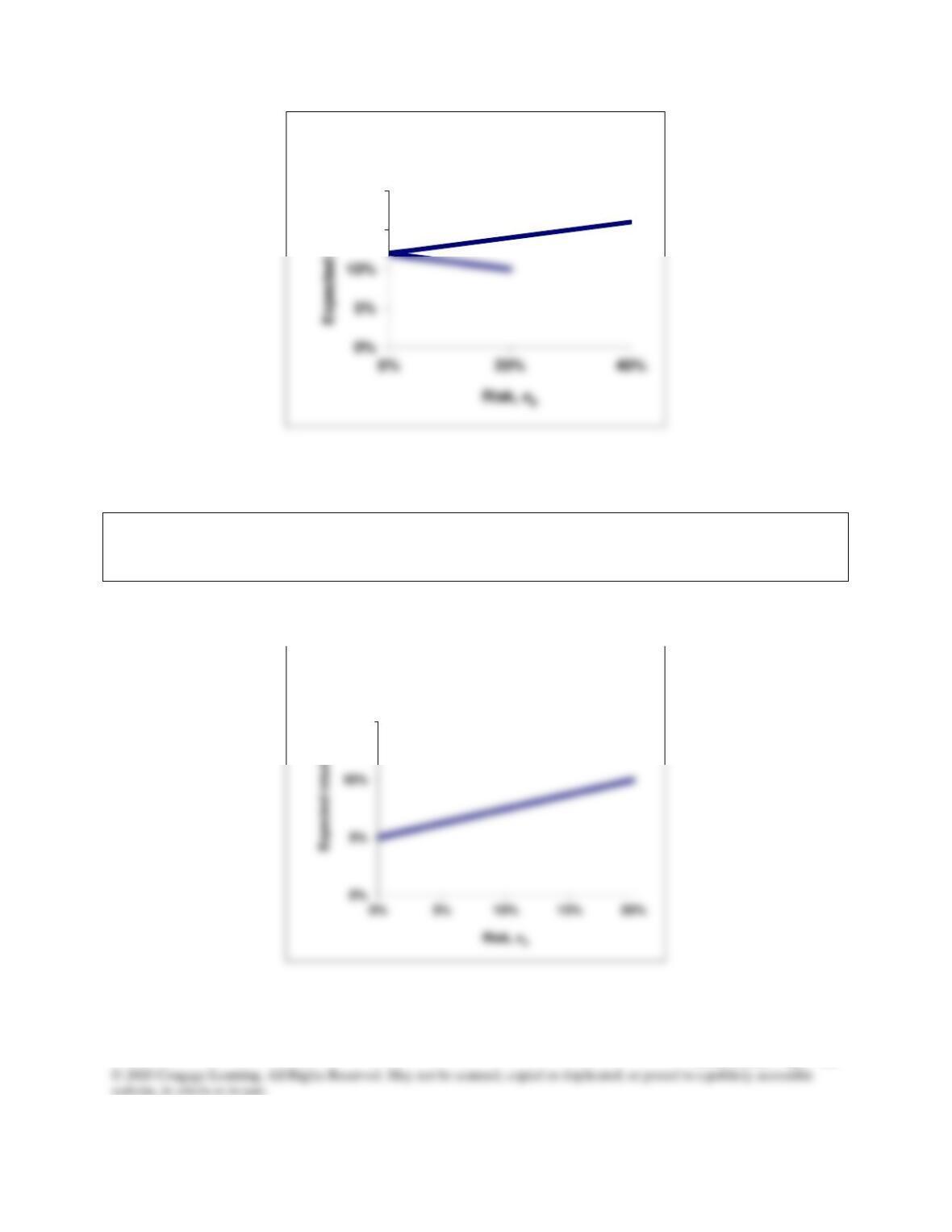
c. Suppose a risk-free asset has an expected return of 5 percent. By definition, its
standard deviation is zero, and its correlation with any other asset is also zero. Using
only asset A and the risk-free asset, plot the attainable portfolios.
Answer:
15%
20%
AB = -1.0: Attainable Set of Risk/Return
Combinations
15%
Attainable Set of Risk/Return
Combinations with Risk-Free Asset
Mini Case: 25 – 14
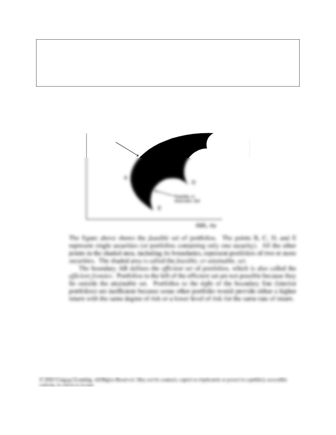
d. Construct a reasonable, but hypothetical, graph which shows risk, as measured
by portfolio standard deviation, on the x axis and expected rate of return on the y
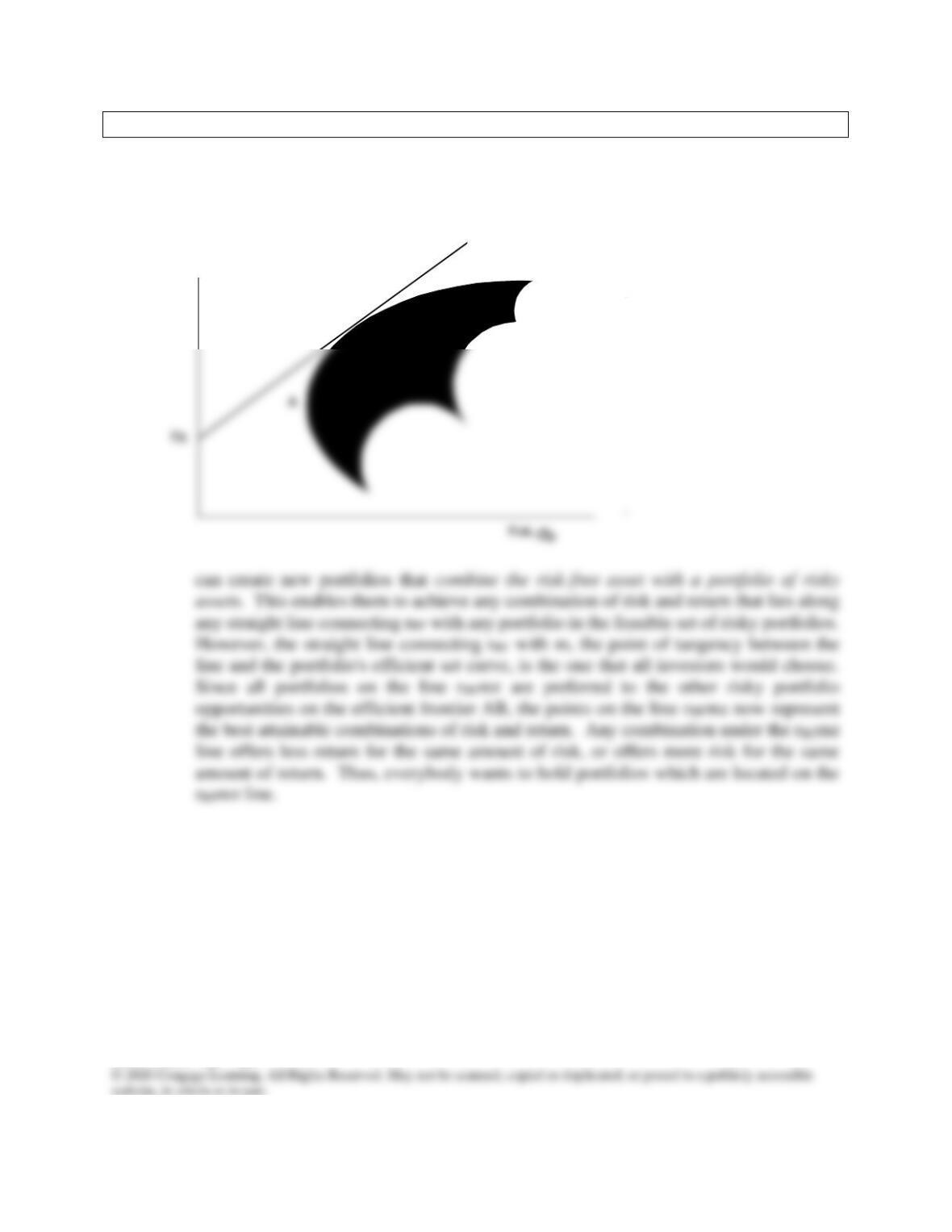
axis. Now add an illustrative feasible (or attainable) set of portfolios, and show
what portion of the feasible set is efficient. What makes a particular portfolio
efficient? Don’t worry about specific values when constructing the graph—
merely illustrate how things look with “reasonable” data.
Answer:
Expected Portfolio
B
C
Return, kp
Efficient Set
(A,B)
^
Expected Portfolio
Return
^
rP
Mini Case: 25 – 15
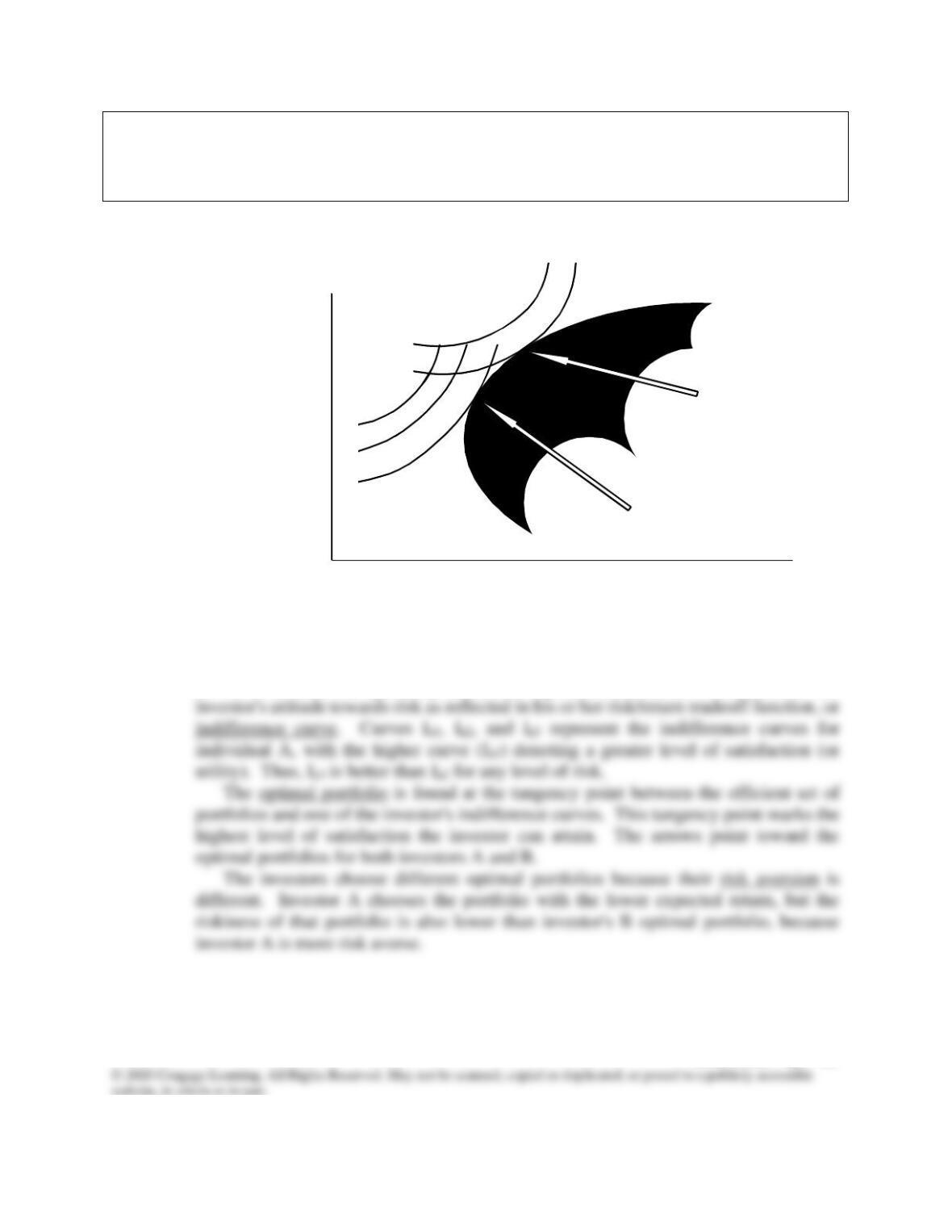
e. Now add a set of indifference curves to the graph created for part B. What do
these curves represent? What is the optimal portfolio for this investor? Finally,
add a second set of indifference curves which leads to the selection of a different
optimal portfolio. Why do the two investors choose different portfolios?
Answer:
The figure above shows the indifference curves for two hypothetical investors, A and
B. To determine the optimal portfolio for a particular investor, we must know the
Expected Portfolio
Risk,
p
A
B
C
D
E
IA3
IA2
IA1
IB2
IB1
Optimal
Portfolio
Investor B
Optimal
Portfolio
Investor A
Return, kp
^
Expected Portfolio
Return,
^
rp
risk, P
Mini Case: 25 – 16
f. Now add the risk-free asset. What impact does this have on the efficient frontier?
Answer: The risk-free asset by definition has zero risk, and hence σ = 0%, so it is plotted on the
vertical axis. Now, given the possibility of investing in the risk-free asset, investors
Expected Portfolio
B
Z
M
Return, kp
^
Expected Portfolio
Return,
^
rp
Mini Case: 25 – 17
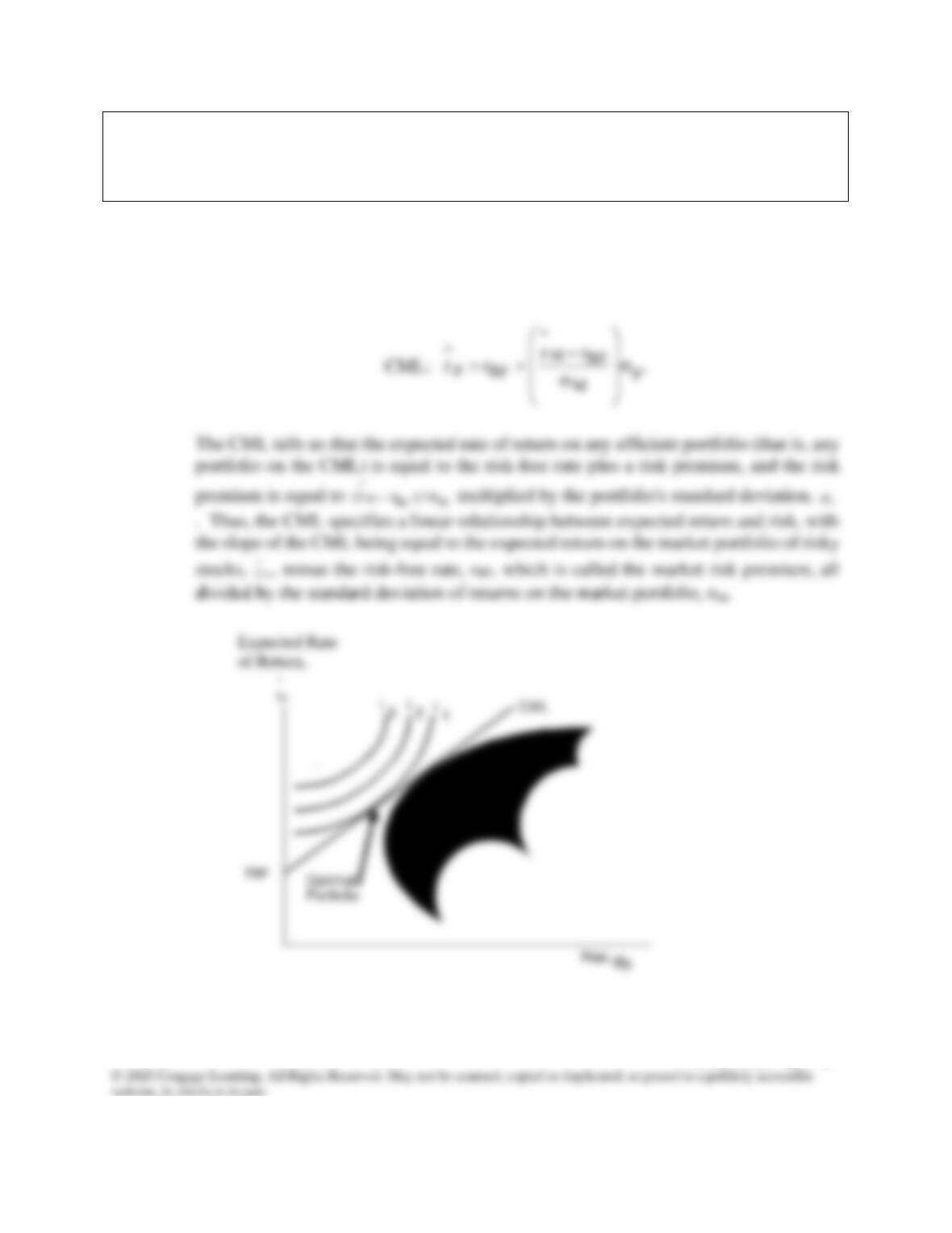
g. Write out the equation for the capital market line (CML) and draw it on the
graph. Interpret the CML. Now add a set of indifference curves, and illustrate
how an investor’s optimal portfolio is some combination of the risky portfolio and
the risk-free asset. What is the composition of the risky portfolio?
Answer: The line rRFMZ in the figure above is called the capital market line (CML). It has an
intercept of rRF and a slope of
MRF
M/)rr( −
. Therefore the equation for the capital
market line may be expressed as follows:
Mini Case: 25 – 18
h. What is the capital asset pricing model (CAPM)? What are the assumptions that
underlie the model?
Answer: The Capital Asset Pricing Model (CAPM) is an equilibrium model which specifies the
relationship between risk and required rates of return on assets when they are held in
well-diversified portfolios. The CAPM requires an extensive set of assumptions:
Mini Case: 25 – 19
i. What is a characteristic line? How is this line used to estimate a stock’s beta
coefficient? Write out and explain the formula that relates total risk, market risk,
and diversifiable risk.
Answer: Betas are calculated as the slope of the characteristic line, which is the regression line
formed by plotting returns on a given stock on the y axis against returns on the general
stock market on the x axis. In practice, 5 years of monthly data, with 60 observations,
would be used, and a computer would be used to obtain a least squares regression line.
Mini Case: 25 – 20
j. What are two potential tests that can be conducted to verify the CAPM? What are
the results of such tests? What is roll’s critique of CAPM tests?
Answer: Since the CAPM was developed on the basis of a set of unrealistic assumptions,
empirical tests should be used to verify the CAPM. The first test looks for stability in
historical betas. If betas have been stable in the past for a particular stock, then its
historical beta would probably be a good proxy for its ex-ante, or expected beta.
Empirical work concludes that the betas of individual securities are not good estimators
Mini Case: 25 – 21
k. Briefly explain the difference between the CAPM and the arbitrage pricing theory
(APT).
Answer: The CAPM is a single-factor model, while the Arbitrage Pricing Theory (APT) can
include any number of risk factors. It is likely that the required return is dependent on