Finance Chapter 18 Attempt to derive risk-adjusted returns that exceed a naive buy-and-hold policy

18 –

1

CHAPTER 18

EVALUATION OF PORTFOLIO PERFORMANCE

Answers to Questions

1. The two major factors would be: (1) attempt to derive risk-adjusted returns that exceed a

naive buy-and-hold policy and (2) completely diversify—i.e., eliminate all unsystematic

2. a) Treynor ratio and Jensen’s alpha measure risk by systematic risk, beta. The Sharp

ratio measure uses total risk, the standard deviation of returns over time. The information

ratio uses the standard deviation of excess returns where excess return is the difference

between the return on a portfolio and its benchmark. The Sortino ratio uses a semi-

deviation measure, including only those returns that fall below a specified minimum

3. For portfolios with R2 values noticeably less than 1.0, it would make sense to compute

both measures. Differences in the rankings generated by the two measures would suggest

4. Jensen’s alpha () is found from the equation Rjt – RFRt == j + j[Rmt – RFRt] +ejt. The

aj indicates whether a manager has superior (j > 0) or inferior (j < 0) ability in market

5. The Information Ratio (IR) is calculated by dividing the average return on the portfolio

less a benchmark return by the standard deviation of the excess return. The IR can be

6. Returns-based measures compare the actual returns on a portfolio to a benchmark. Sharpe

and Treynor are simple measures, comparing portfolio returns to a risk-free rate. The

information ratio and Sortino can use the returns of the benchmark portfolio as the

standard of comparison. Another type of returns-based analysis is returns-based style

7. The difference by which a manager’s overall actual return beats his/her overall

benchmark return is termed the total value-added return and decomposes into an

allocation effect and a selection effect. The former effect measures differences in weights

8.

8(a).

Benchmark

Explain two different weaknesses of using each of the

benchmarks to measure the performance of the portfolio.

Market

Index

• A market index may exhibit survivorship bias; firms that have

gone out of business are removed from the index resulting in a

performance measure that overstates the actual performance had

the failed firms been included.

• A market index may exhibit double counting that arises because

of companies owning other companies and both being represented

in the index.

• It is often difficult to exactly and continually replicate the

holdings in the market index without incurring substantial trading

costs.

• The chosen index may not be an appropriate proxy for the

management style of the managers.

• The chosen index may not represent the entire universe of

securities (e.g., S&P 500 Index represents 65–70 percent of U.S.

equity market capitalization).

• The chosen index may have a large capitalization bias (e.g., S&P

500 has a large capitalization bias).

• The chosen index may not be investable. There may be securities

in the index that cannot be held in the portfolio.

Benchmark

Normal

Portfolio

• This is the most difficult performance measurement method to

develop and calculate.

• The normal portfolio must be continually updated, requiring

substantial resources.

• Consultants and clients are concerned that managers who are

involved in developing and calculating their benchmark portfolio

may produce an easily-beaten normal portfolio making their

performance appear better than it actually is.

able to invest in the median manager portfolio.

18 –

4

(Continued)

• Such a benchmark may be ambiguous. The names and weights of

the securities constituting the benchmark are not clearly

delineated.

• The benchmark is not constructed prior to the start of an

evaluation period; it is not specified in advance.

• A manager universe may exhibit survivorship bias; managers that

have gone out of business are removed from the universe resulting

in a performance measure that overstates the actual performance

had those managers been included.

8b)i.

The Sharpe ratio is calculated by dividing the portfolio risk premium, (i.e., actual

portfolio return minus risk-free return) by the portfolio standard deviation of return.

Sharpe Ratio = (Rp – Rf)/p

The Treynor measure is calculated by dividing the portfolio risk premium (i.e., actual

portfolio return minus risk-free return) by the portfolio beta.

8(b).ii.

The Sharpe ratio assumes that the relevant risk is total risk and measures excess return

per unit of total risk.

18 –

5

9.

9(a). The basic procedure in portfolio evaluation is to compare the return on a managed

portfolio to the return expected on an unmanaged portfolio having the same risk, via use

of the CAPM. That is, expected return (Rp) is calculated from:

Rp = Rf + p(Rm – Rf)

9(b). The benchmark error often occurs because the unmanaged portfolio used in the

evaluation process is not “optimized.” That is, market indices, such as the S&P 500,

9(c). The main ingredients are that the true risk-free rate is lower than the measured risk-free

9(d). The response depends upon one’s beliefs about whether these portfolios represent the true

market portfolio. The DJIA is comprised of only 30 industrial stocks; S&P 500 includes

9(e). Defense of CAPM: it is valid as a normative theory as it describes the proper measure of

risk (systematic risk, not total risk or another risk definition) and it shows what the

18 –

6

10. When measuring the performance of an equity portfolio manager, overall returns can be

related to a common total risk or systematic risk. Factors influencing the returns achieved

by the bond portfolio manager are more complex. In order to evaluate performance based

CHAPTER 18

Answers to Problems

1(a).

.03

.07.10

1.30

.10

.13

.10

.07.20

S

60.1

.05

.08

0.05

.07.15

S

Q

P

−

==

−

=

==

−

=

18 –

8

2.

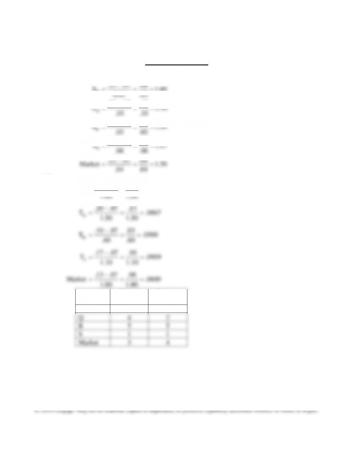
2(a). The Treynor measure (T) relates the rate of return earned above the risk-free rate to the

portfolio beta during the period under consideration. Therefore, the Treynor measure

shows the risk premium (excess return) earned per unit of systematic risk:

0.60

1.00

The Treynor measure examines portfolio performance in relation to the security market

line (SML). Because the portfolio would plot above the SML, it outperformed the S&P

500 Index. Because T was greater than TM, 6.7 percent versus 6.0 percent, respectively,

Sharpe Measure Performance Relative to the Market (S&P 500)

Market (S&P 500)

2(b). The Treynor measure assumes that the appropriate risk measure for a portfolio is its

systematic risk, or beta. Hence, the Treynor measure implicitly assumes that the portfolio

being measured is fully diversified. The Sharpe measure is similar to the Treynor

measure except that the excess return on a portfolio is divided by the standard deviation

of the portfolio.

For perfectly diversified portfolios (that is, those without any unsystematic or specific

3(a). Portfolio MNO enjoyed the highest degree of diversification because it had the highest R2

(94.8 percent). The statistical logic behind this conclusion comes from the CAPM, which

says that all fully diversified portfolios should be priced along the security market line.

3(b). Note the mean returns are net of the risk-free rate. Doing the calculations we obtain:

Fund Treynor Sharpe Jensen

DEF 0.715(5) 0.619(5) -0.053(5)

JKL 1.262(2) 0.915(3) 0.355(2)

3(c).

Fund t(alpha)

DEF -0.2789(5)

JKL 1.6136(4)

Only GHI and MNO have significantly positive alphas at a 95% level of confidence.

4(a). Overall performance (Fund 1) = 26.40% – 6.20% = 20.20%

4(b). E(Ri) = 6.20 + (15.71 – 6.20)

4(c)(i). Selectivity1 = 20.2% – 12.85% = 7.35%

4(c)(ii).Ratio of total risk1 = 1/m = 20.67/13.25 = 1.56

18 –

11

4(c)(iii). Net Selectivity = Selectivity – Diversification

4(d). Even accounting for the added cost of incomplete diversification, Fund 1’s performance

was above the market line (best performance), while Fund 2’s performance fell below the

line.

5.

a.

Year

Mgr X

Return

Mgr Y Return

1

-1.5

-6.5

2

-1.5

-3.5

3

-1.5

4

-1.0

3.5

5

0.0

4.5

6

4.5

6.5

7

6.5

7.5

8

8.5

9

13.5

12.5

10

17.5

13.5

Average

4.5

Std Dev

6.90

6.63

Semi-dev

0.65

4.20

Semi-deviation considers only the returns that are below the average.

b.

Sharpe ratio: (average return minus risk-free rate) / standard deviation

Mgr X:

0.435

Mgr Y:

0.452

Best performer

c.

Sortino ratio: (average return minus minimum acceptable return)/semi-

deviation

Mgr X:

4.602

Best performer

Mgr Y:

0.714

d. The Sharpe and Sortino measures should provide the same performance ranking when

the return distributions are symmetrical for the funds or managers under consideration.

18 –

12

6.

6(a)(i). .6(-5) + .3(-3.5) + .1(0.3) = -4.02%

7.

7(a). Overall, both managers added value by mitigating the currency effects present in the Index.

Both exhibited an ability to “pick stocks” in the markets they chose to be in (Manager B

in particular). Manager B used his opportunities not to be in stocks quite effectively (via

the cash/bond contribution to return), but neither of them matched the passive index in

picking the country markets in which to be invested (Manager B in particular).

7(b). The column reveals the effect on performance in local currency terms after adjustment

for movements in the U.S. dollar and, therefore, the effect on the portfolio. Currency

gains/losses arise from translating changes in currency exchange rates versus the U.S.

8.

18 –

13

8(a). Evaluation begins with selection of the appropriate benchmark against which to measure

the firms’ results:

Firm A. The Aggregate Index and “Managers using the Aggregate Index” benchmark are

Performance has been good (30 basis points ahead of the index and in the second quartile

of manager results) but not as good as Firm A’s showing during this relatively short

measurement period.

8(b). Firm A does not show an observable degree of security selection skill (-10 basis points);

nor does it appear to be managing in line with its stated marketlike approach. Some large

nonmarketlike bets are driving return production (e.g., duration bets, +100 basis points;

8(c). Firm C produced the best results because its style and its expertise were confirmed by the

9(a). Dollar-Weighted Return

Manager L:

500,000 = -12,000/(1+r) – 7,500/(1+r)2– 13,500/(1+r)3 – 6,500/(1+r)4– 10,000/(1+r)5+

18 –

14

9(b). Time-weighted return

Manager L:

Periods HPR

1 [(527,000 – 500,000) – 12,000]/500,000 = .03

2 [(530,000 – 527,000) – 7,500]/527,000 = -.0085

Manager M:

Periods HPR

1 [(692,000 – 700,000) + 35,000]/700,000 = .03857

2 [(663,000 – 692,000) + 35,000]/692,000 = .00867

EV – (1 – DW)(Contribution)

9(c). Dietz approximation method = – 1

BV + (DW)(Contribution)

Manager M:

Periods HPY

1 [(692,000 – (1 -.50)(-35,000)]/[700,000 + (.50)(-35,000)] – 1

= (692,000 + 17,500/(700,000 – 17,500) – 1 = 709,500/682,500 – 1 = .0396

2 (663,000 – (1 -.50)(-35,000)]/[692,000 + (.50)(-35,000)] – 1

10 (a) Average Return AFNDX-RF = 1.637

Average Return SPX-RF = 1.540

10(b)

SUMMARY OUTPUT

Regression Statistics

Multiple R

0.77359

R Square

0.598442

Adjusted R

Square

0.588146

Standard

Error

3.682119

Observation

s

41

ANOVA

df

SS

MS

F

Significan

18 –

16

ce F

Regression

1

788.0144

788.014

4

58.1217

2

3.03E-09

Residual

39

528.7621

13.558

Total

40

1316.776

Coefficien

ts

Standard

Error

t Stat

P-value

Lower

95%

Upper

95%

Lower

95.0%

Upper

95.0%

Intercept

0.222915

0.604211

0.36893

5

0.71417

1

-0.99922

1.44504

6

–

0.99922

1.44504

6

SPX-RFR

0.918015

0.120415

7.62376

3.03E-

09

0.674453

1.16157

8

0.67445

3

1.16157

8

(1) One-factor Jensen’s alpha coefficient 0.2229

(2) Beta coefficient 0.9180

10 (c) Treynor’s ratio performance measure

10 (d) Although the portfolio has a low risk premium per unit of risk as indicated by the Sharpe

10 (e) The tracking error (TE) for AFNDX on a monthly basis is 5.738 and on an annualized

10 (f) The information ratio (IF) = 1.637/5.738 = 0.2853. This represents the manager’s average

18 –

17

10(g).

SUMMARY OUTPUT

Regression Statistics

Multiple R

0.834821

R Square

0.696926

Adjusted R

Square

0.672352

Standard

Error

3.284201

Observation

s

41

ANOVA

df

SS

MS

F

Significan

ce F

Regression

3

917.6953

305.898

4

28.3607

5

1.07E-09

Residual

37

399.0812

10.7859

8

Total

40

1316.776

Coefficien

ts

Standard

Error

t Stat

P-value

Lower

95%

Upper

95%

Lower

95.0%

Upper

95.0%

Intercept

0.081039

0.540695

0.14988

0.88167

4

-1.01451

1.17659

1

–

1.01451

1.17659

1

Excess Mkt

0.895537

0.131509

6.80970

2

5.09E-

08

0.629075

1.162

0.62907

5

1.162

SMB

0.041786

0.129354

0.32303

8

0.74848

5

-0.22031

0.30388

3

–

0.22031

0.30388

3

HML

-0.18187

0.19729

–

0.92185

0.36257

7

-0.58162

0.21787

5

–

0.58162

0.21787

5

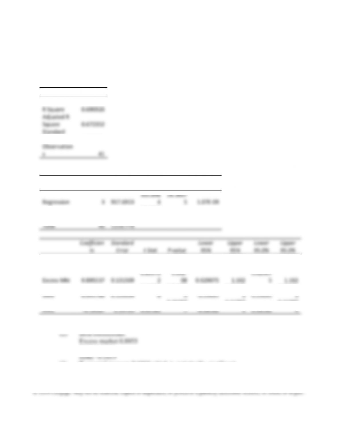
(1) Intercept coefficient is 0.08104 is statistically insignificant.

SMB 0.0418

(3) R-squared measure 0.6969 which is statistically significant.

18 –

18