17-11 a. The inputs to the Black and Scholes option pricing model are P = 5, X = 2, rRF = 6%,
σ = 50%, and t = 2 years. Given these inputs, the value of a call option is calculated
as:
b. The debt must therefore be worth 5-3.29 = $1.71 million. Its yield is
%1.881.0171.1/0.2 ==−
.
Answers and Solutions: 17 – 18
17-12 a. HVU,3 =
07.013.0
)07.1( 40$
−
= $713.33.
c. TS = (Interest expense)(T)
HVU,3 =
07.013.0
)07.1( 0.4$
−
= $71.33.
d. 0 1 2 3 4
| | | | |
3.2 3.6 4.0
rsU = 13%
g = 7%
Answers and Solutions: 17 – 19

SOLUTION TO SPREADSHEET PROBLEM
17-13 The detailed solution for the problem is available in the file IFM12 Ch17 P13 Build a
Model Solution.xls on the textbook’s Web site.
Answers and Solutions: 17 – 20

MINI CASE
David Lyons, CEO of Lyons Solar Technologies, is concerned about his firm’s level of debt
financing. The company uses short–term debt to finance its temporary working capital
needs, but it does not use any permanent (long–term) debt. Other solar technology
companies average about 30 percent debt, and Mr. Lyons wonders why they use so much
more debt, and what its effects are on stock prices. To gain some insights into the matter, he
poses the following questions to you, his recently hired assistant:
a. Who were Modigliani and Miller (MM), and what assumptions are embedded in
the MM and Miller models?
Answer: Modigliani and Miller (MM) published their first paper on capital structure (which
assumed zero taxes) in 1958, and they added corporate taxes in their 1963 paper.
Modigliani won the Nobel Prize in economics in part because of this work, and most
subsequent work on capital structure theory stems from MM. Here are their
assumptions:
• Firms’ business risk can be measured by σEBIT, and firms with the same degree of
risk can be grouped into homogeneous business risk classes.
Mini Case: 17 – 21

b. Assume that firms U and L are in the same risk class, and that both have EBIT =
$500,000. Firm U uses no debt financing, and its cost of equity is rsU = 14%. Firm
L has $1 million of debt outstanding at a cost of rd = 8%. There are no taxes.
Assume that the MM assumptions hold, and then:
1. Find v, s, rs, and WACC for firms U and L.
Answer: First, we find Vu and VL:
To find rsL, it is necessary first to find the market values of firm L’s debt and equity.
The value of its debt is stated to be $1,000,000. Therefore, we can find s as follows:
We know from Proposition I that the WACC must be WACC = rsU = 14.0% for all
firms in this risk class, regardless of leverage, but this can be verified using the WACC
formula:
Mini Case: 17 – 22
b. 2. Graph (a) the relationships between capital costs and leverage as measured by
D/V, and (b) the relationship between value and D.
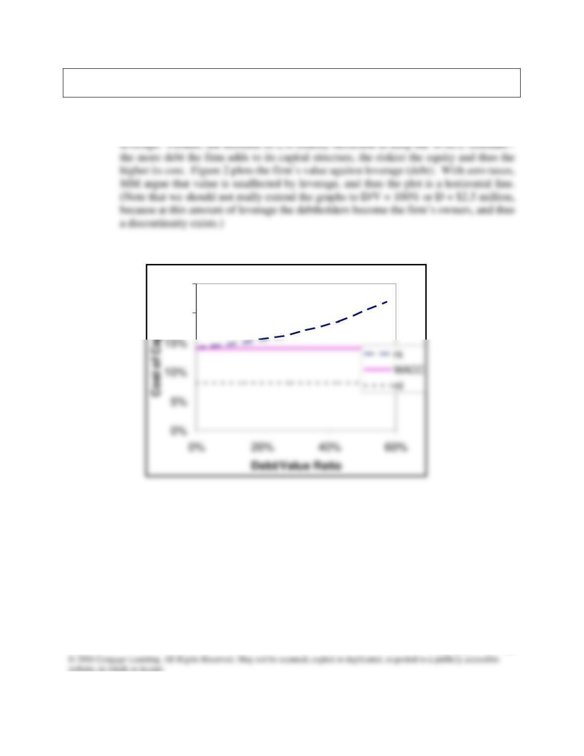
Answer: Figure 1 plots capital costs against leverage as measured by the debt/value ratio. Note
that, under the MM no-tax assumption, rd is a constant 8 percent, but rs increases with
Figure 1
Without Taxes
20%
25%
Mini Case: 17 – 23
c. Using the data given in part B, but now assuming that firms L and U are both
subject to a 40 percent corporate tax rate, repeat the analysis called for in B(1)
and B(2) under the MM with-tax model.
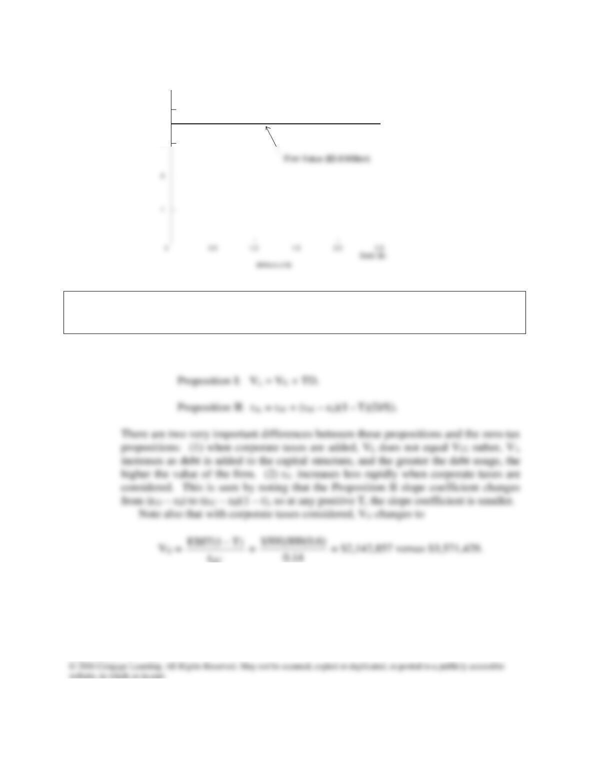
Answer: With corporate taxes added, the MM propositions become:
sU
4
3
Value of Firm, V
V
U
V
L
($)
Figure 2
Mini Case: 17 – 24
This represents a 40% decline in value, and it is logical, because the 40% tax rate takes
away 40% of the income and hence 40% of the firm’s value.
Looking at VL, we see that:
now,
The WACC is lower for the levered firm than for the unlevered firm when corporate
taxes are considered.
Figure 3 below plots capital costs at different D/V ratios under the MM model with
corporate taxes. Here the WACC declines continuously as the firm uses more and more
Mini Case: 17 – 25
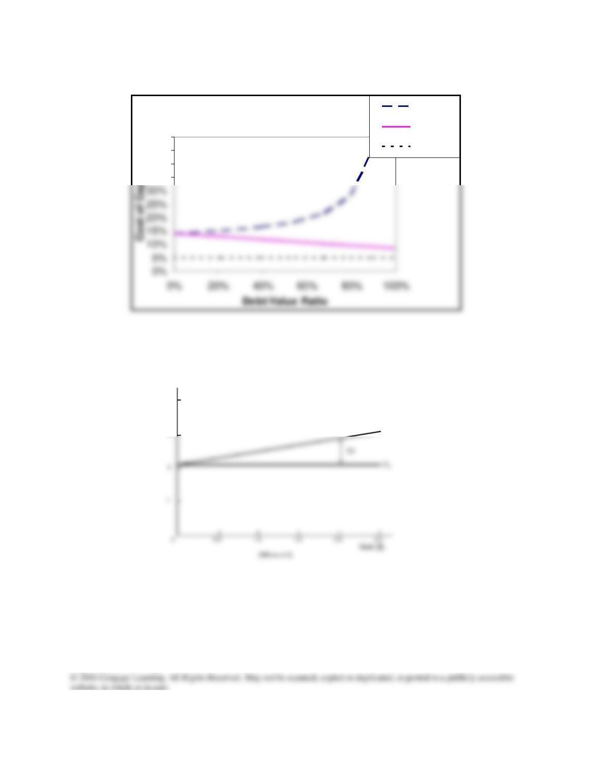
Figure 3
4
3
Value of Firm, V
V
L
($)
Figure 4
With Taxes
35%
40%
45%
50%
rs
WACC
rd x (1-T)
Mini Case: 17 – 26
d. Now suppose investors are subject to the following tax rates:
TD = 30% and TS = 12%.
1. What is the gain from leverage according to the miller model?
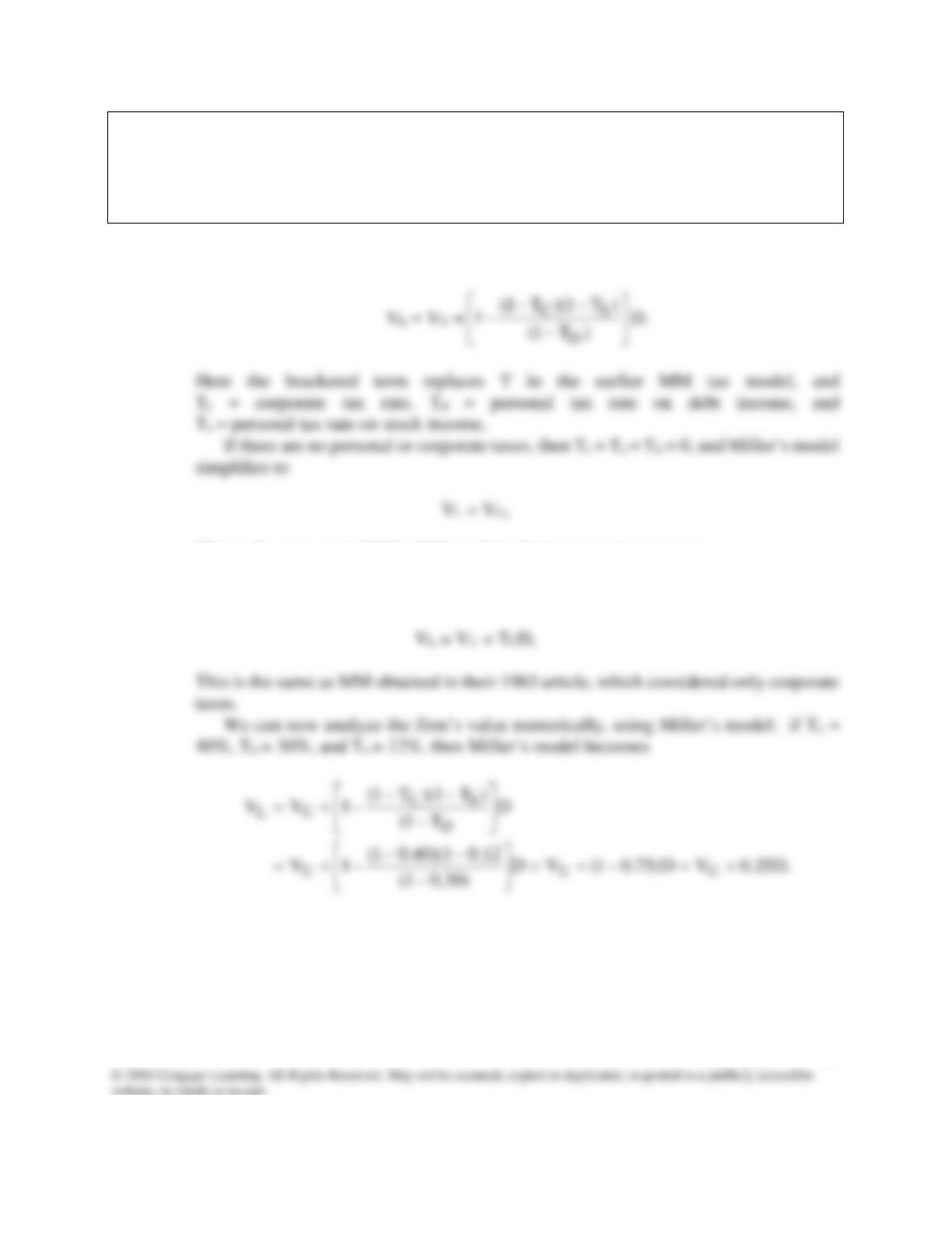
Answer: To begin, note that Miller’s Proposition I is stated as follows:
This is the same as in MM’s 1958 model, which assumed zero taxes.
If there are corporate taxes, but no personal taxes, then Ts = Td = 0, and Miller’s
model simplifies to
Mini Case: 17 – 27
d. 2. How does this gain compare to the gain in the MM model with corporate taxes?
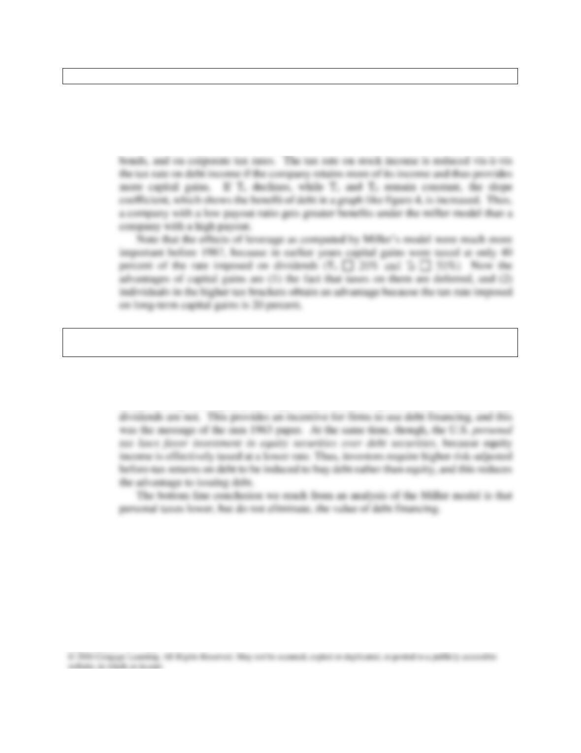
Answer: If only corporate taxes were considered, then
VL = VU + TCD = VU + 0.40D.
The net effect depends on the relative effective tax rates on income from stocks and
d. 3. What does the Miller model imply about the effect of corporate debt on the value
of the firm, that is, how do personal taxes affect the situation?
Answer: The addition of personal taxes lowers the value of debt financing to the firm. The
underlying rationale can be explained as follows: the U.S. corporate tax laws favor
debt financing over equity financing, because interest expense is tax deductible while
Mini Case: 17 – 28
e. What capital structure policy recommendations do the three theories (MM
without taxes, MM with corporate taxes, and Miller) suggest to financial
managers? Empirically, do firms appear to follow any one of these guidelines?
Answer: In a zero tax world, MM theory says that capital structure is irrelevant—it has no impact
on firm value. Thus, one capital structure is as good as another. With corporate but
f. Suppose that Firms U and L are growing at a constant rate of 7% and that the
investment in net operating assets required to support this growth is 10% of EBIT.
Use the compressed adjusted present value (APV) model to estimate the value of
U and L. Also estimate the levered cost of equity and the weighted average cost of
capital.
Answer: If a firm is growing, the assumptions that MM made are violated. The extension to the
MM model shows how growth affects the value of the debt tax shield and the cost of
capital. The first difference in this situation is that the appropriate discount rate for the
Mini Case: 17 – 29

If there is $1,000,000 in debt then:
The value of l = the value of U + value of debt tax shield
The value of the (growing) debt tax shield = rdTD/(rsU – g)
= 0.08(0.40)(1,000,000)/(0.14 – 0.07)
= $457,143
To calculate the new levered cost of equity:
rsL = rsU + (rsU – rd)(D/S)
= 14% + (14% – 8%)(1,000,000/3,028,571)
g. Suppose the expected free cash flow for Year 1 is $250,000 but it is expected to
grow unevenly over the next 3 years: FCF2 = $290,000 and FCF3 = $320,000, after
which it will grow at a constant rate of 7%. The expected interest expense at Year
1 is $80,000, but it is expected to grow over the next couple of years before the
capital structure becomes constant: Interest expense at Year 2 will be $95,000, at
Year 3 it will be $120,000 and it will grow at 7% thereafter. What is the estimated
horizon unlevered value of operations (i.e., the value at Year 3 immediately after
the FCF at Year 3)? What is the current unlevered value of operations? What is
the horizon value of the tax shield at Year 3? What is the current value of the tax
shield? What is the current total value? The tax rate and unlevered cost of equity
remain at 40% and 14%, respectively.
Mini Case: 17 – 30
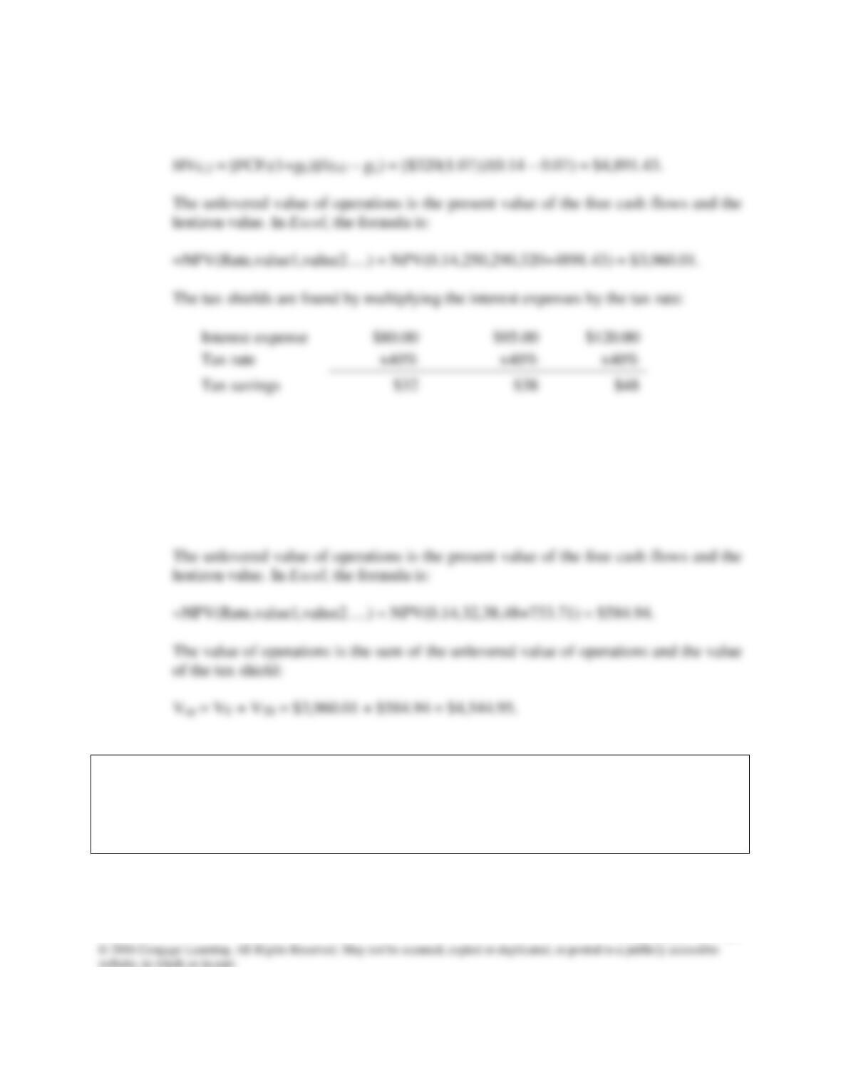
Answer: The unlevered horizon value of operations can be found by applying the constant
growth formula:
The horizon value of the tax shield can be found by applying the constant growth
formula:
HVTS,3 = [TS3(1+gL)]/(rsU – gL) = [$48(1.07)]/(0.14 – 0.07) = $733.71.
h. Suppose there is a large probability that L will default on its debt. For the purpose
of this example, assume that the value of L’s operations is $4 million (the value of
its debt plus equity). Assume also that its debt consists of 1–year, zero coupon
bonds with a face value of $2 million. Finally, assume that L’s volatility, σ is 0.60
and that the risk–free rate rRF is 6%.
Mini Case: 17 – 31
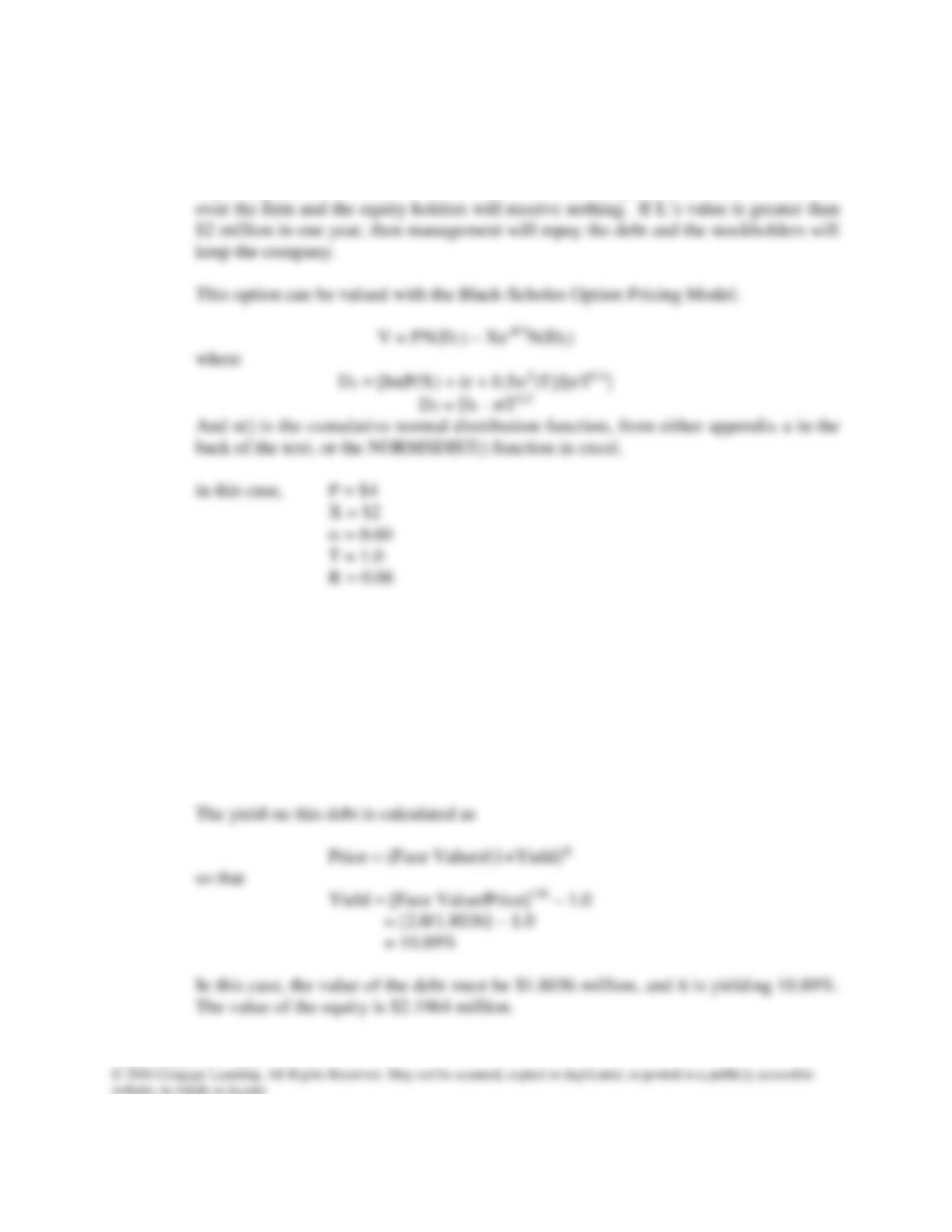
Answer: L’s equity can be considered as a call option on the total value of l with an exercise
price of $2 million, and an expiration date in one year. If the value of L’s operations
is less than $2 million in a year, then L’s management will not be able to make its
required payment on the debt, and the firm will be bankrupt. The debtholders will take
and calculating,
D1 = 1.552
D2 = 0.9552
N(D1) = 0.9491
N(D2) = 0.8303
and V = $2.1964 million.
This leaves debt value of $4 million – $2.1964 million = $1.8036 million.
Mini Case: 17 – 32

Mini Case: 17 – 33
i. What is the value of L’s stock for volatilities between 0.20 and 0.95? What
incentives might the manager of L have if she understands this relationship?
What might debtholders do in response?
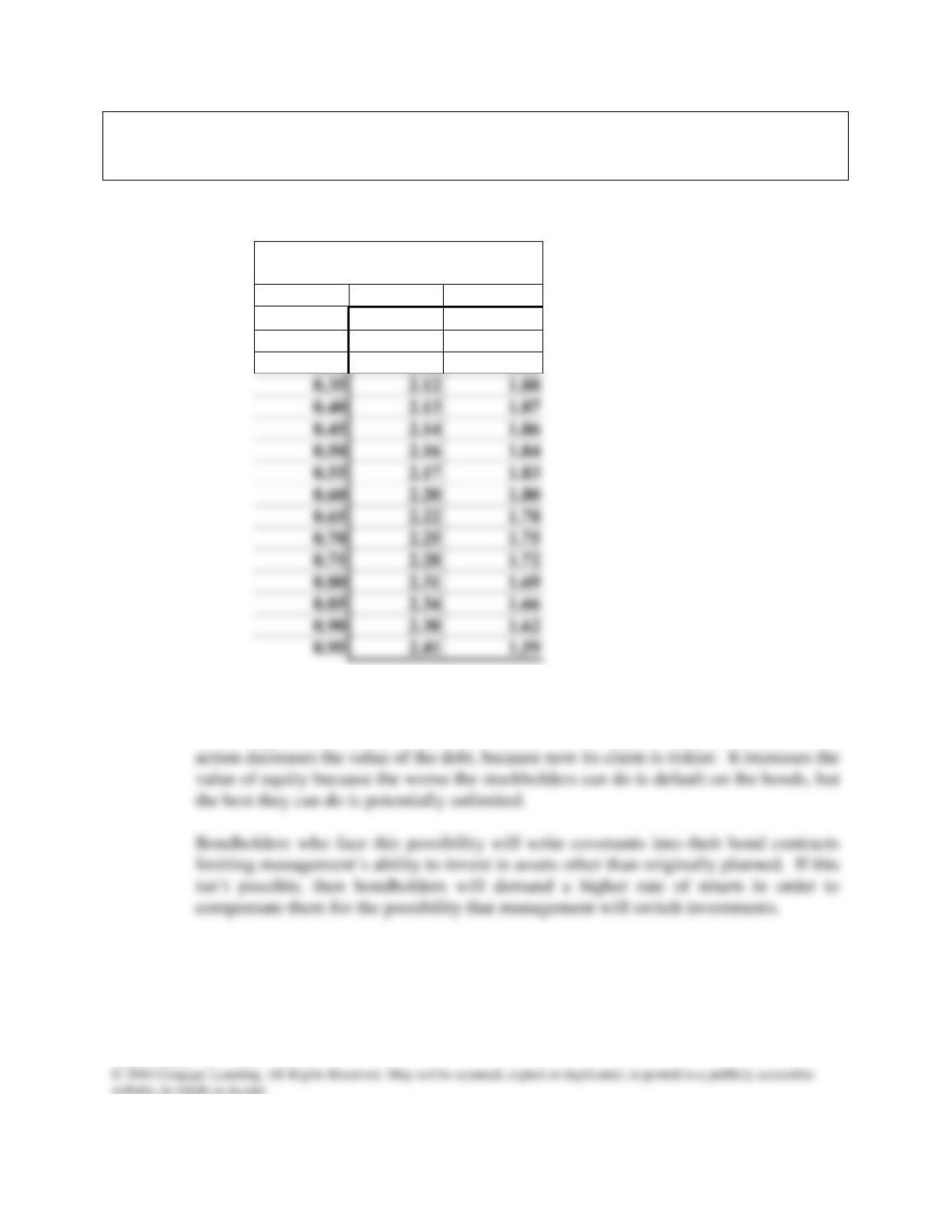
Answer: The mini case model shows the calculations for the table below.
Value of Stock and Debt
for Different Volatilities
Volatility
Equity
Debt
0.20
2.12
1.88
0.25
2.12
1.88
0.30
2.12
1.88
The value of the equity increases as the volatility increases—and the value of the debt
decreases as well. A manager who knows this may choose to invest the proceeds from
borrowing in assets that are riskier than usual. This is called “bait and switch.” This
Mini Case: 17 – 34
0.35
2.12
1.88
0.40
2.13
1.87
0.45
2.14
1.86
0.50
2.16
1.84
0.60
2.20
1.80
0.65
2.22
1.78
0.70
2.25
1.75
0.75
2.28
1.72
0.80
2.31
1.69
0.85
2.34
1.66
0.90
2.38
1.62
0.95
2.41
1.59