g. What does the empirical evidence say about capital structure theory? What are
the implications for managers?
Answer: Tax benefits are important. At the optimal capital structure, $1 debt adds about $0.10
to $0.20 to value on average. For the average firm financed with 25% to 30% debt,
this adds about 3% to 6% to the total value. However, these results were based on
periods prior to the TCJA and may now overstate the value added by debt.
Sometimes companies will deliberately increase debt to above target to take
advantage of unexpected investment opportunity.
After big stock price run ups, the debt ratio falls, but firms tend to issue equity
instead of debt. This is inconsistent with the trade-off model, inconsistent with the
pecking order theory, but is consistent with the windows of opportunity hypothesis.
Many firms, especially those with growth options and asymmetric information
problems, tend to maintain excess borrowing capacity.
h. With the above points in mind, now consider the optimal capital structure for
PizzaPalace.
h. (1) For each capital structure under consideration, calculate the levered beta, the cost
of equity, and the WACC.
Answer: MM theory implies that beta changes with leverage. bu is the beta of a firm when it
has no debt (the unlevered beta). Hamada’s equation provides the beta of a levered
firm: bL = bU [1 + (1 – T)(D/S)]. For example, to find the cost of equity for wd = 20%,
we first use Hamada’s equation to find beta:
b = bU [1 + (1 – T)(D/S)]
= 1.0 [1 + (1-0.25) (20% / 80%)]
Next, find the WACC. For example, the WACC for wd = 20% is:
WACC = wd (1-T) rd + ws rs
WACC = 0.2 (1 – 0.25) (8%) + 0.8 (13.13%)
WACC = 11.7%
h. (2) Now calculate the corporate value.
Answer: For example, suppose that wd = 20% is:
FCF = NOPAT – Investments in operating capital
= EBIT(1 − T) – Investments in operating capital
= $120(1 – 0.25) – $0 = $90.
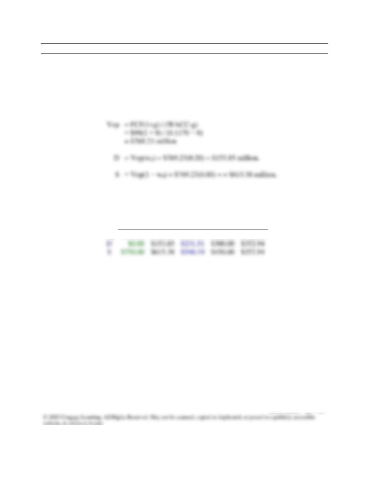
Repeating this for all capital structures gives the following table:
wd
0%
20%
30%
40%
50%
Vop
$750.00
$769.23
$771.70
$750.00
$705.88
$153.85
$231.51
$300.00
$352.94
$750.00
$615.38
$540.19
$450.00
$352.94
i. Describe the recapitalization process and apply it to PizzaPalace. Calculate the
resulting the value of the debt that will be issued, the resulting market value of
equity, the price per share, the number of shares repurchased, and the remaining
shares. Considering only the capital structures under analysis, what is
PizzaPalace’s optimal capital structure?
Answer:
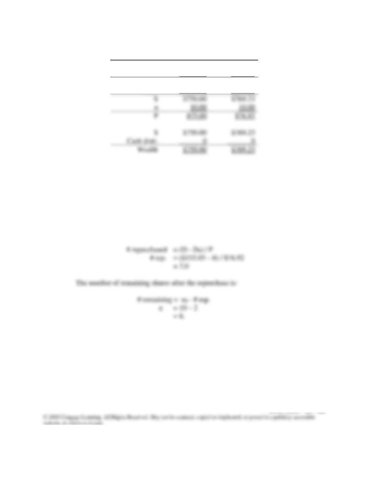
The situation before the recap is:
Before
Debt
Vop
$750.00
+ ST Inv.
0
$750.00
0
$750.00
$750.00
0
$750.00
The stock price is $75 and the total wealth of shareholders is $750 million.
Before Debt
After Debt,
Before Rep.
Vop
$750.00
$769.23
+ ST Inv.
0
$153.85
VTotal
$750.00
$923.08
− Debt
0
$153.85
$750.00
$769.23
$750.00
$769.23
0
0
$750.00
$769.23
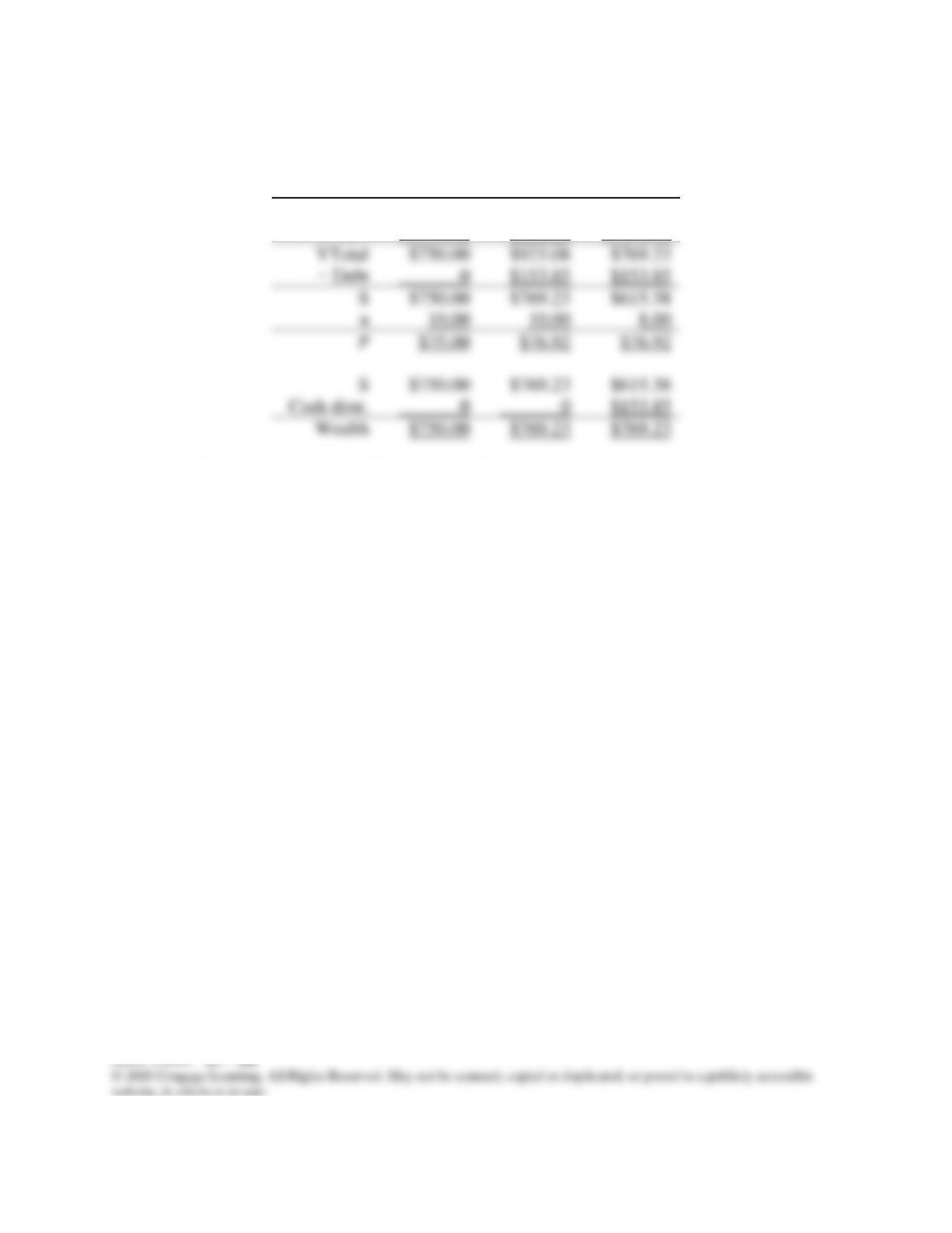
Notice that the stock price increases and the wealth of shareholders increases.
The repurchase itself will not change the stock price. If investors thought that the
repurchase would increase the stock price, they would all purchase stock the day
before, which would drive up its price. If investors thought that the repurchase would
decrease the stock price, they would all sell short the stock the day before, which
would drive down the stock price.
The number of shares repurchased is:
Before
Debt
After
Debt,
Before
Rep.
After Rep.
Vop
$750.00
$769.23
$769.23
+ ST Inv.
0
$153.85
0
$750.00
$923.08
$769.23
0
$153.85
$153.85
$750.00
$769.23
$615.38
$750.00
$769.23
$615.38
0
0
$153.85
$750.00
$769.23
$769.23
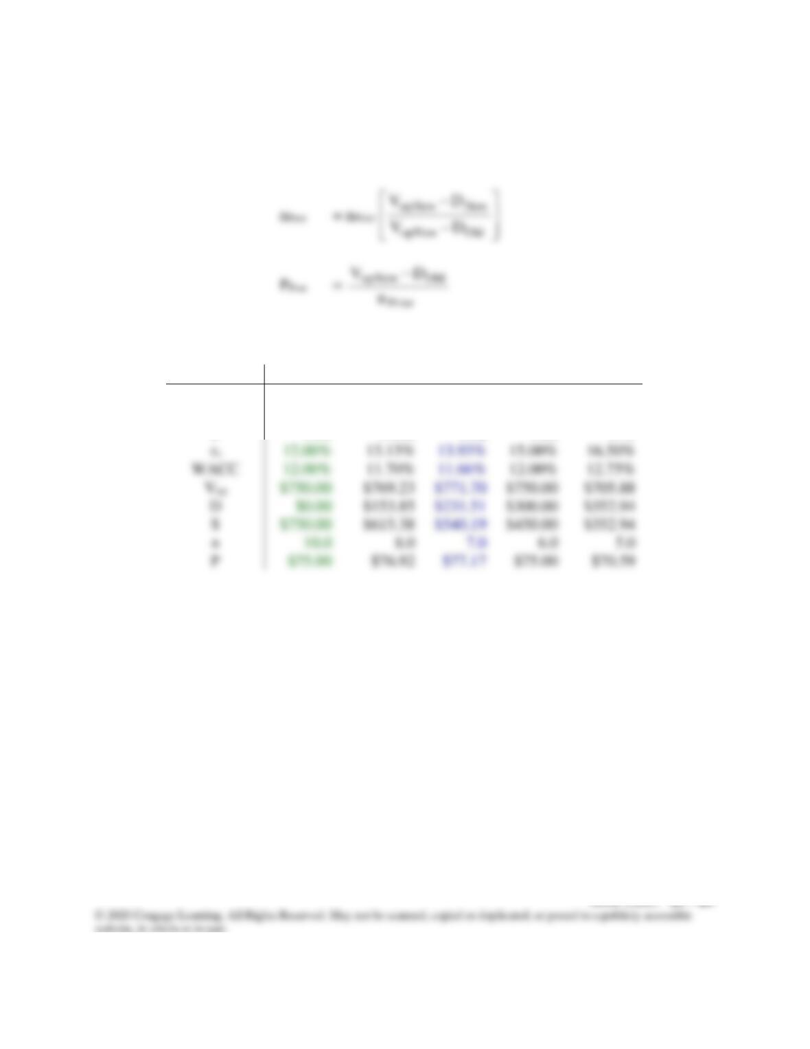
Notice that the value of the equity declines as more debt is issued, because debt is
used to repurchase stock. But the total wealth of shareholders is the value of stock
after the recap plus the cash received in repurchase, and this total is not changed by
the repurchase.
There are some shortcuts we can take to find the values of S, P, and n after the
repurchase:
S = (1 – wd) Vop
We apply these relationships for each possible capital structure:
wd
0%
20%
30%
40%
50%
rd
0.0%
8.0%
8.5%
10.0%
12.0%
ws
100%
80%
70%
60%
50%
b
D
The optimal capital structure is for wd = 30%. This gives the highest corporate value,
the lowest WACC, and the highest stock price per share. But notice that wd = 20% is
very similar to the optimal solution; in other words, the optimal range is pretty flat.
j. Liu Industries is a highly levered firm. Suppose there is a large probability that
Liu will default on its debt. The value of Liu’s operations is $4 million. The firm’s
debt consists of 1–year, zero coupon bonds with a face value of $2 million. Liu’s
volatility, σ, is 0.60 and the risk-free rate rRF is 6%. Because Liu’s debt is risky, its
equity is like a call option and can be valued with the Black-Scholes Option Pricing
Model (OPM). (See Chapter 8 for details of the OPM.)
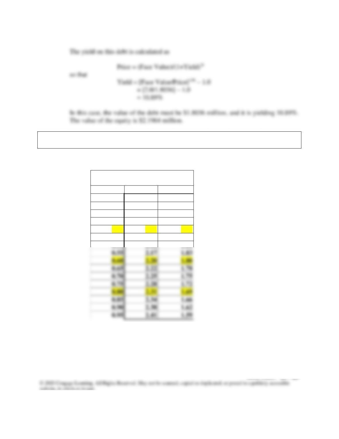
j. (1) What are the values of Liu’s stock and debt? What is the yield on the debt?
Answer: Liu’s equity can be considered as a call option on the total value of l with an exercise
price of $2 million, and an expiration date in one year. If the value of Liu’s operations
is less than $2 million in a year, then Liu’s management will not be able to make its
required payment on the debt, and the firm will be bankrupt. The debtholders will take
over the firm and the equity holders will receive nothing. If Liu’s value is greater than
$2 million in one year, then management will repay the debt and the stockholders will
keep the company.
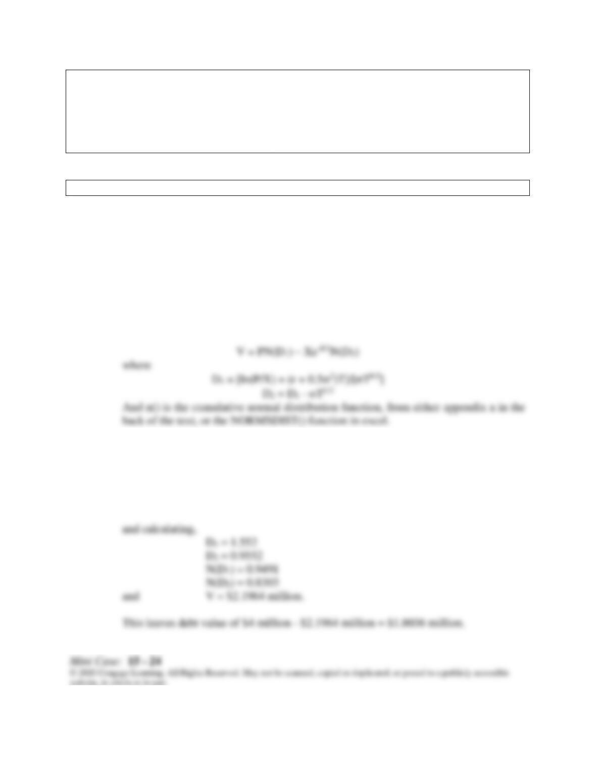
This option can be valued with the Black-Scholes Option Pricing Model:
in this case, P = $4
X = $2
= 0.60
T = 1.0
R = 0.06
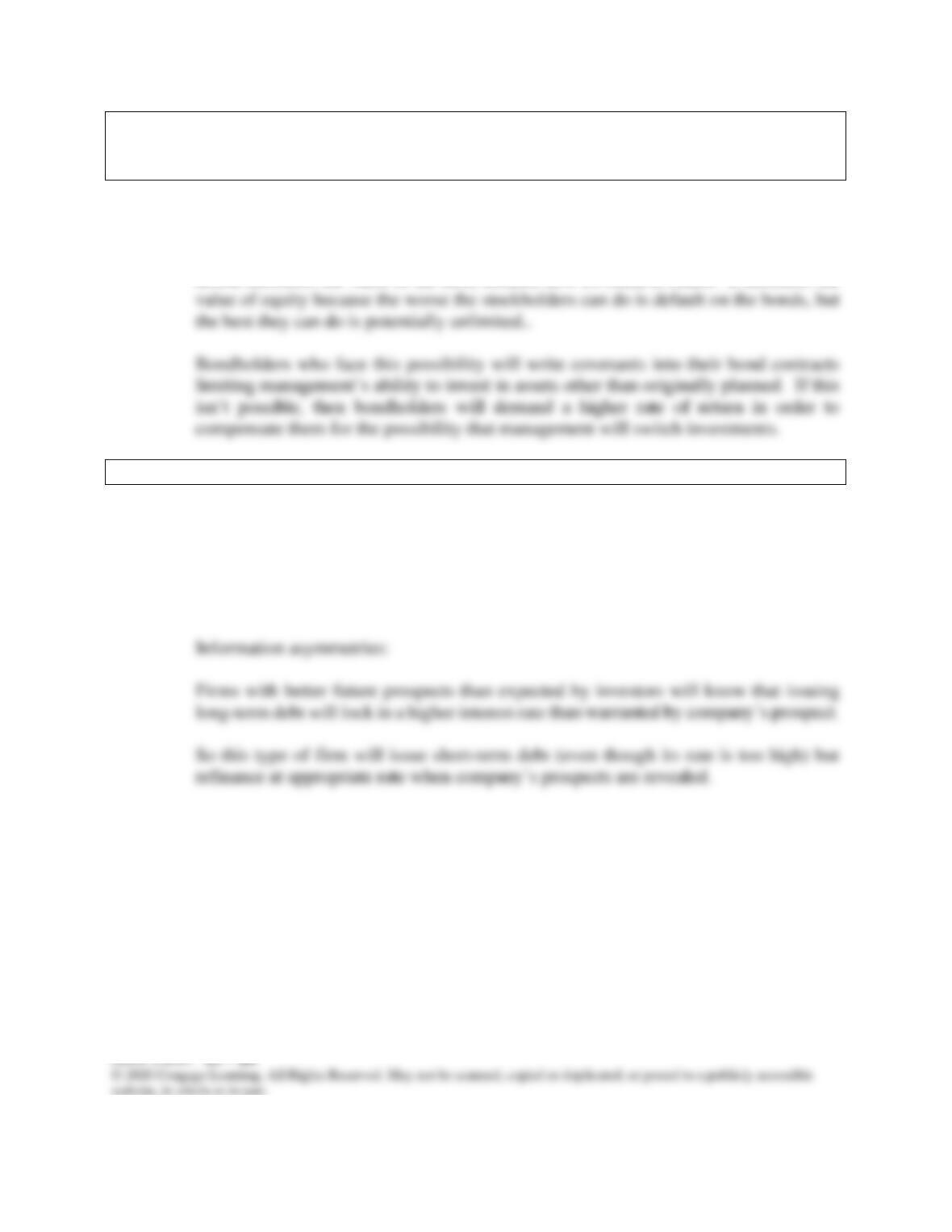
j. (2) What are the values of Liu’s stock and debt for volatilities of 0.40 and 0.80? What
are yields on the debt?
Answer: The mini case model shows the calculations for the table below.
Value of Stock and Debt
for Different Volatilities
Volatility
Equity
Debt
0.20
2.12
1.88
0.25
2.12
1.88
0.30
2.12
1.88
0.35
2.12
1.88
0.40
2.13
1.87
0.45
2.14
1.86
0.50
2.16
1.84
0.55
2.17
1.83
0.60
2.20
1.80
0.65
2.22
1.78
0.70
2.25
1.75
0.75
2.28
1.72
0.80
2.31
1.69
0.85
2.34
1.66
0.90
2.38
1.62
0.95
2.41
1.59
j. (3) What incentives might the manager of Liu have if she understands the
relationship between equity value and volatility? What might debtholders do in
response?
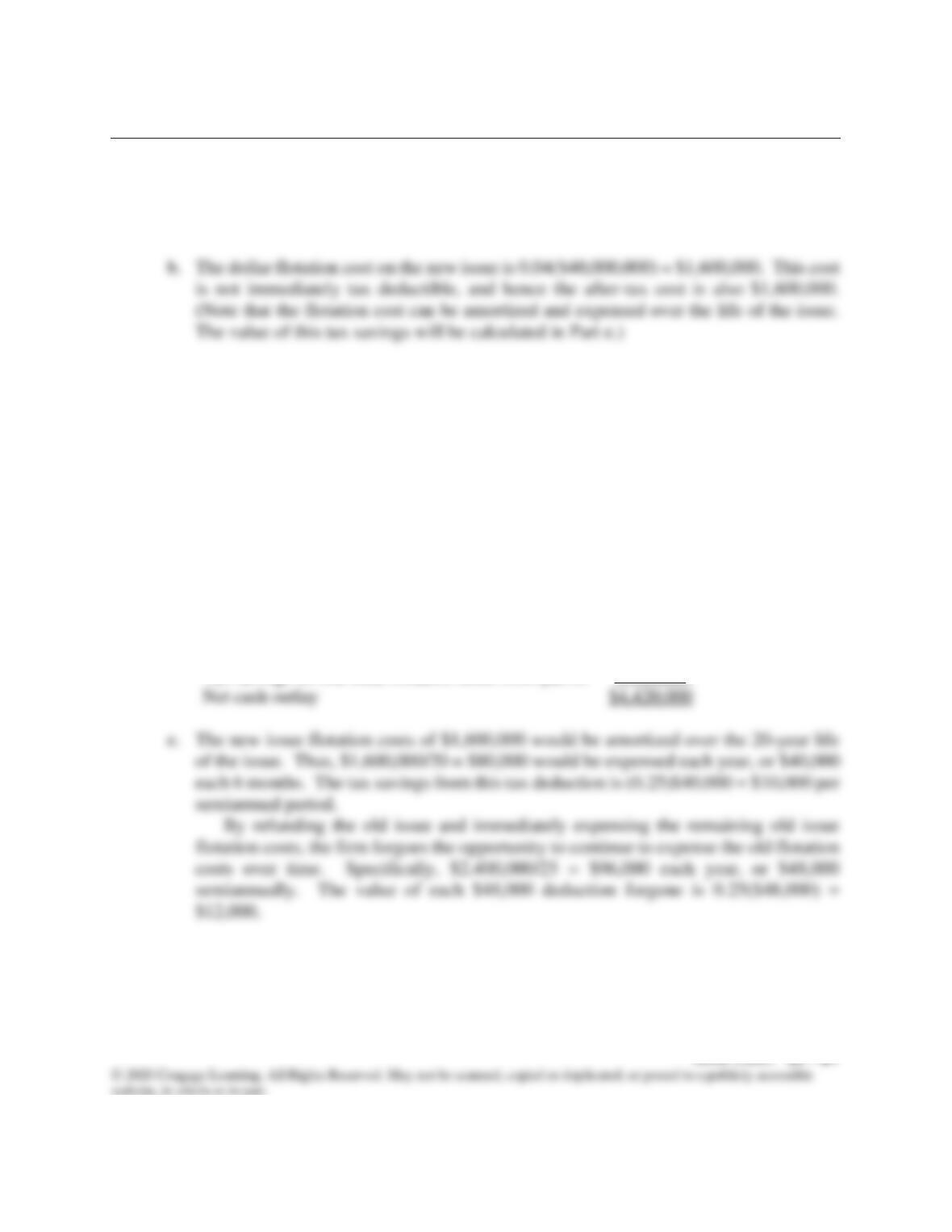
Answer: The value of the equity increases as the volatility increases—and the value of the debt
decreases as well. A manager who knows this may choose to invest the proceeds from
borrowing in assets that are riskier than usual. This is called “bait and switch.” This
k. How do companies manage the maturity structure of their debt?
Answer: Factors that influence the decision to issue long-term bonds rather than short-term debt:
Maturity matching:
Finance long-term assets with long-term debt
Finance short-term assets with short-term debt.
SOLUTIONS TO END–OF-WEB EXTENSION PROBLEMS
15B-1 a. Since the call premium is 11 percent, the total premium is 0.11($40,000,000) =
$4,400,000. However, this is a tax deductible expense, so the relevant after-tax cost is
$4,400,000(1 – T) = $4,400,000(0.75) = $3,300,000.
c. The flotation costs on the old issue were 0.06($40,000,000) = $2,400,000. These costs
were deferred and are being amortized over the 25-year life of the issue, and hence
$2,400,000/25 = $96,000 are being expensed each year, or $48,000 each 6 months.
Since the bonds were issued 5 years ago, (5/25)($2,400,000) = $480,000 of the flotation
costs have already been expensed, and (20/25)($2,400,000) = $1,920,000 remain
unexpensed.
If the issue is refunded, the unexpensed portion of the flotation costs can be
immediately expensed, and this would result in a tax savings of T($1,920,000) =
0.25($1,920,000) = $480,000.
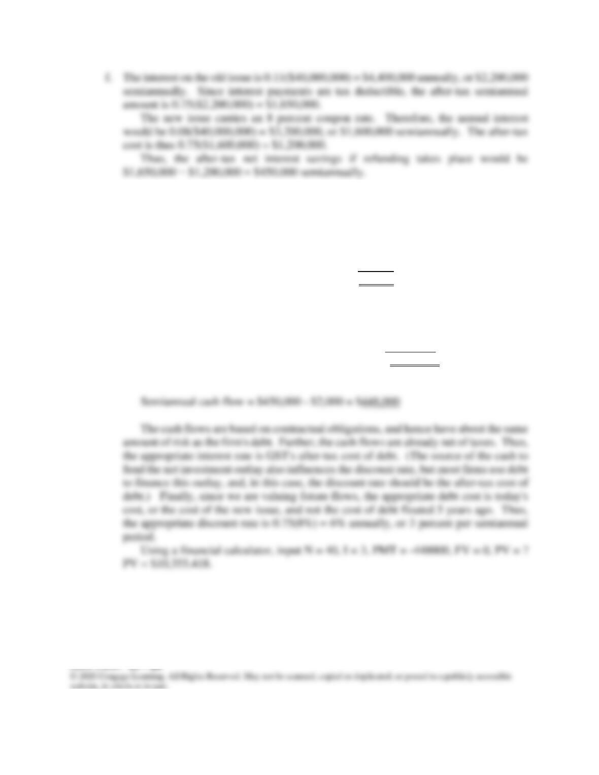
d. The net after-tax initial cash outlay is shown below:
Old issue call premium from part a: $3,300,000
New issue flotation cost from part b: 1,600,000
g.
Semiannual Flotation Cost Tax Effects:
Semiannual tax savings on new flotation: $10,000
Tax benefits lost on old flotation: (12,000)
Net amortization tax effects ($ 2,000)
Semiannual after-tax Interest Savings Due To Refunding:
Semiannual after-tax interest on old bond: $1,650,000
Semiannual after-tax interest on new bond: (1,200,000)
Net semiannual after-tax interest savings $ 450,000
h.
PV of net benefits from part g: $10,355,418
Initial cash flow from part d: −$4,420,000
Refunding NPV $5,935,418
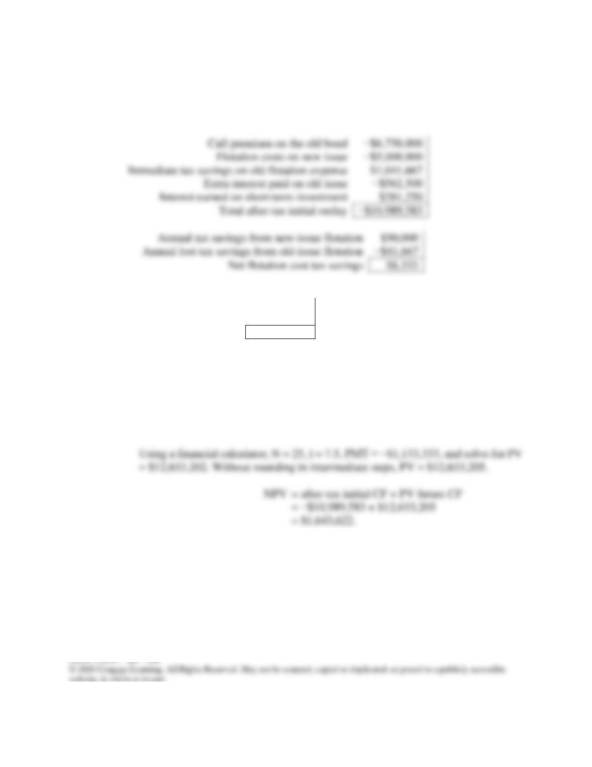
15B-2 a. Investment outlay required to refund the issue (all figures after-tax):
−$10,989,583
Annual lost tax savings from old-issue flotation
−$41,667
Interest on old bond
$6,750,000
Interest on new bond
−$5,625,000
Net interest savings
$1,125,000
Total annual CF = Net flotation cost tax savings+ Net interest savings
= $8,333 + $1,125,000 = $1,133,333
After-tax interest rate = 10%(1 − 0.25) = 7.5%
b. The company should consider what interest rates might be next year. If there is a high
probability that rates will drop below the current rate, it may be more advantageous to
refund later versus now. If there is a high probability that rates will increase, the firm
should act now to refund the old issue. Also, the company should consider how much
ill will is created with investors if the issue is called. If Mullet is highly dependent on
a small group of investors, it would want to avoid future difficulty in obtaining

financing. However, bond issues are callable after a certain time and investors expect
them to be called if rates drop considerably.
SOLUTIONS TO WEB EXTENSION SPREADSHEET PROBLEMS
15B-3 The detailed solution for the spreadsheet problem, Solution for Ch15 Web15B P03 Build
a Model.xlsx, is available on the textbook’s Web site.