Finance Chapter 14 Just use traditional DCF approaches to capital budgeting

Chapter 14

Real Options

ANSWERS TO BEGINNING-OF–CHAPTER QUESTIONS

14-1 Financial options deal with securities like stocks and debt instruments, whereas real options

deal with physical assets like capital budgeting projects. There are many different types of

real options, ranging from those related to whole plants to options on commodities such as

oil, electricity, gas, and copper. We focused primarily on real options as they relate to

The text discusses several approaches to dealing with real options:

• Ignore them. Just use traditional DCF approaches to capital budgeting.

• Recognize them and deal with them in a qualitative, judgmental manner.

• Take a decision tree, or scenario analysis, approach, and find the NPV of a project with

In the chapter BOC spreadsheet model, we analyze a project’s timing option using the

first 4 procedures. The Tool Kit for the chapter extends the analysis to growth, flexibility,

and abandonment options.

Some real options are inherent in capital budgeting, but others can be created. For

Answers and Solutions: 14 – 1

14-2 See the BOC model for an example of a scenario analysis and a Black–Scholes analysis for

an investment timing option. Similar analyses for growth and abandonment options are

contained the chapter Tool Kit.

Some controversy exists regarding the use of decision trees versus formal option

pricing models. The primary advantage of the decision tree approach is that it is relatively

easy to implement, and it is easy to explain to decision makers. One doesn’t even need to

discuss options per se—simply calculate the project’s NPV with and without the option,

The bottom line, to us, is that if one focuses just on a particular decision, such as the

project in our BOC model, where we consider the decision the decision to proceed now or

to wait, there is no significant advantage to either method. The decision tree approach is

more straightforward and easier to explain to managers, but both lead to the same decision

Answers and Solutions: 14 – 2

14-3 Several factors should be considered. First, if projects are never undertaken, then they

never provide any benefits in the form of NPV, so companies do need to invest at some

point. Second, and related to the first point, a dollar of cash flow today is better than a

14-4 In general, each of these options would increase the expected NPV and reduce the standard

deviation and coefficient of variation of the expected NPV, which would mean a lower

14-5 The answer to this question has been discussed in the preceding answers. The company

could delay the decision to get more information on the demand for power, it could build

in flexibility with regard to fuel used (gas, oil, or coal), and it could consider the

possibility of abandonment if things turned out badly. Companies in the power industry

ANSWERS TO END-OF-CHAPTER QUESTIONS

14-1 a. Real options occur when managers can influence the size and risk of a project’s cash

flows by taking different actions during the project’s life. They are referred to as real

b. Investment timing options give companies the option to delay a project rather than

implement it immediately. This option to wait allows a company to reduce the

14-2 Postponing the project means that cash flows come later rather than sooner; however,

14-3 Timing options make it less likely that a project will be accepted today. Often, if a firm can

delay a decision, it can increase the expected NPV of a project.

Answers and Solutions: 14 – 4

SOLUTIONS TO END-OF-CHAPTER PROBLEMS

14-1 a. 0 1 2 20

├─────┼─────┼────── • • • ────┤

–20 3 3 3

b. Wait 1 year:

PV @

0 1 2 3 21 Yr. 1

Tax imposed | | | | • • • |

50% Prob. 0 –20 2.2 2.2 2.2 15.45

r= 13%

Answers and Solutions: 14 – 5

14-2 a. 0 1 2 3 4

├─────┼─────┼─────┼─────┤

–8 4 4 4 4

NPV = $4.6795 million.

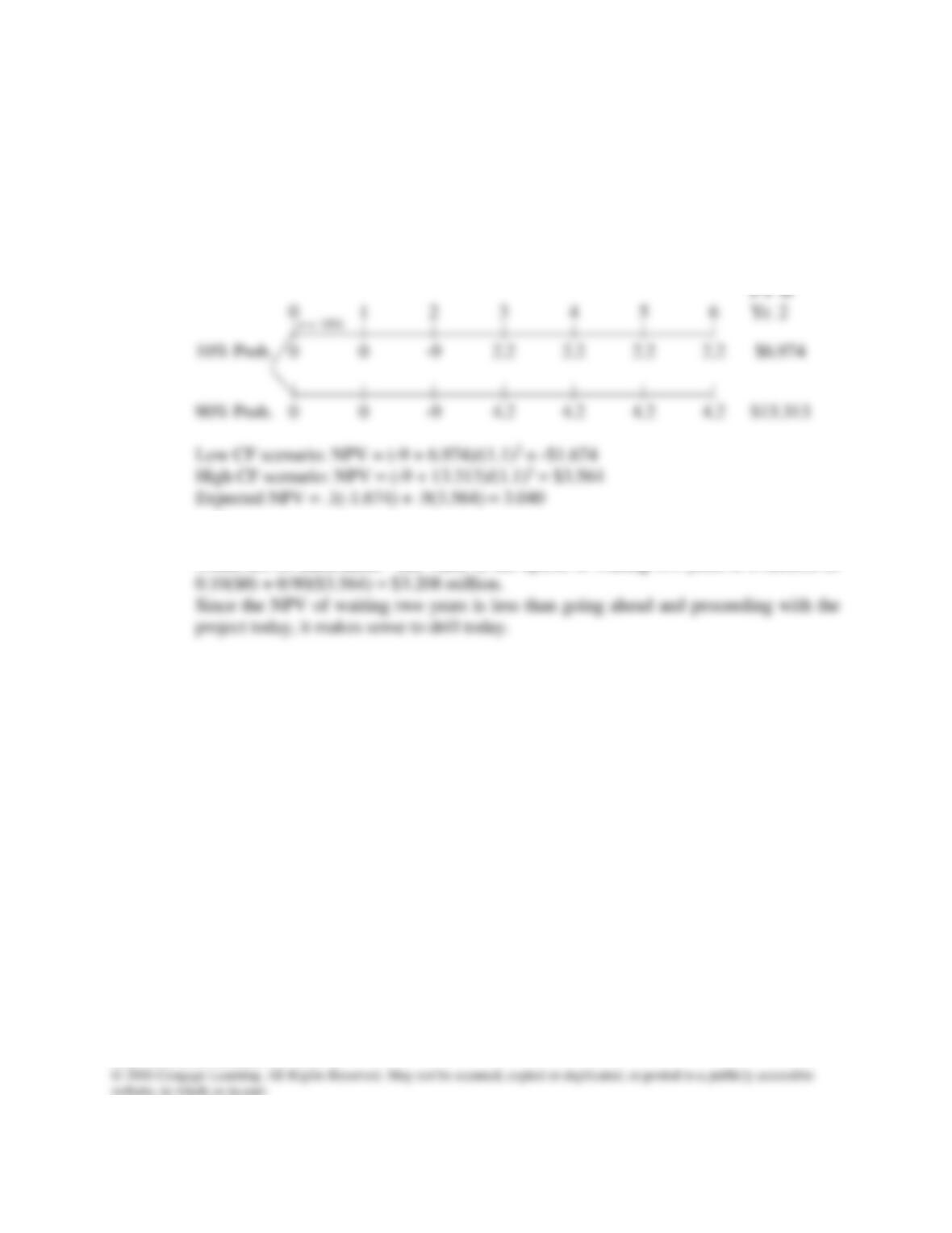
b. Wait 2 years:

If the cash flows are only $2.2 million, the NPV of the project is negative and, thus,

would not be undertaken. The value of the option of waiting two years is evaluated as

10%

Answers and Solutions: 14 – 6

14-3 a. 0 1 2 20

├─────┼─────┼────── • • • ────┤

–300 40 40 40

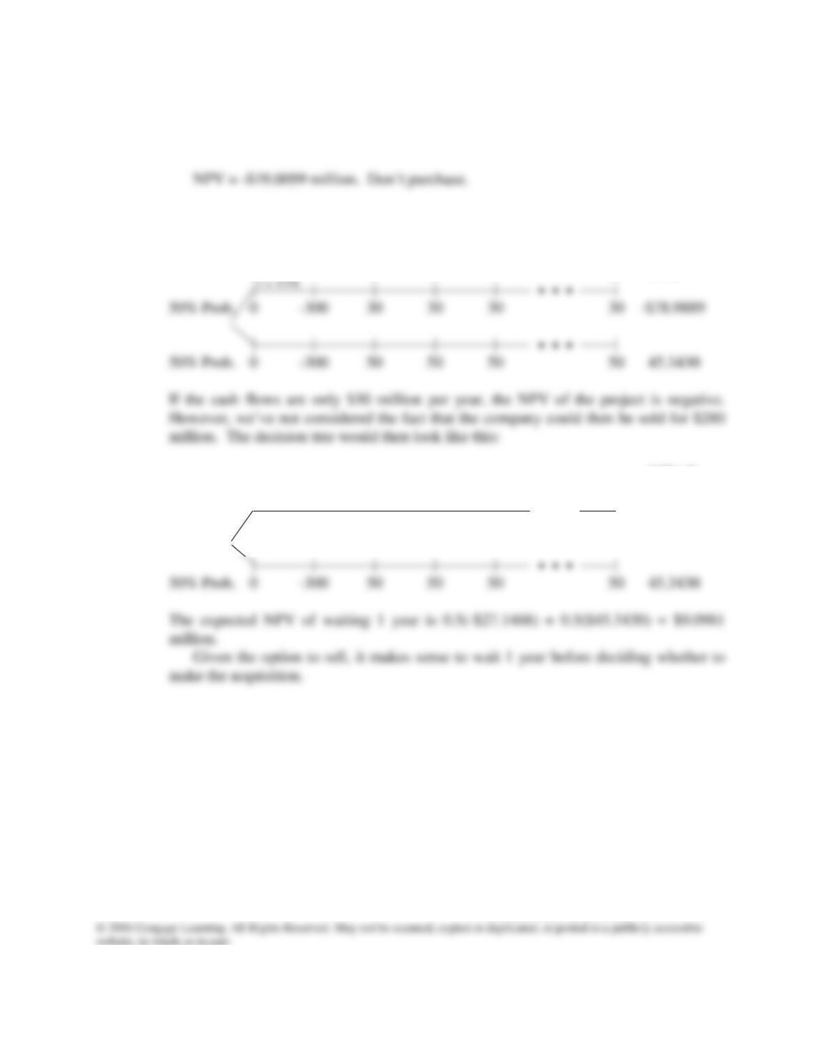
b. Wait 1 year:

NPV @

0 1 2 3 4 21 Yr. 0

NPV @

0 1 2 3 4 21 Yr. 0

| | | | | • • • |

50% Prob. 0 –300 30 30 + 280 0 0 –$27.1468

13%

r = 13%

Answers and Solutions: 14 – 7

14-4 a. 0 1 14 15

b. 0 1 14 15

| | • • • | |

–6,200,000 1,200,000 1,200,000 1,200,000

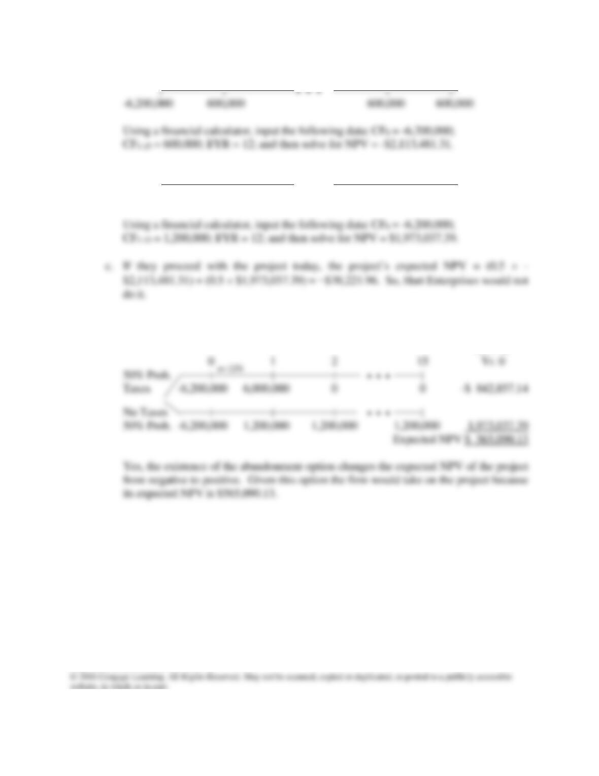
d. Since the project’s NPV with the tax is negative, if the tax were imposed the firm would

abandon the project. Thus, the decision tree looks like this:

NPV @

12%

Answers and Solutions: 14 – 8

e. NPV @

0 1 Yr. 0

50% Prob. | |

Taxes NPV = ? –1,500,000 $ 0.00

+300,000 = NPV @ t = 1

r = 12%

}wouldn’t do

Answers and Solutions: 14 – 9

14-5

a.

0 1 2

40% Prob. | | |

Good –20,000 25,000 25,000 NPV = 23,388

b.

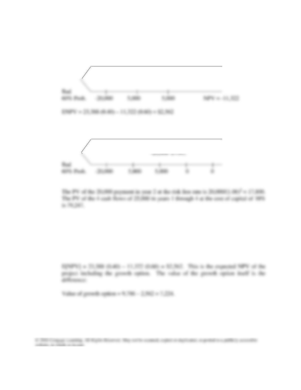
0 1 2 3 4

Good –20,000 25,000 25,000 25,000 25,000

The NPV of the top row is 79,247 – 20,000 – 17,800 = 41,447.

The NPV of the bottom row is still –11,332, as it was in part a.

The expected NPV, E[NPV], is 41,447 (0.40) –11,332 (0.60) = $9,786.

r = 10%

Answers and Solutions: 14 – 10

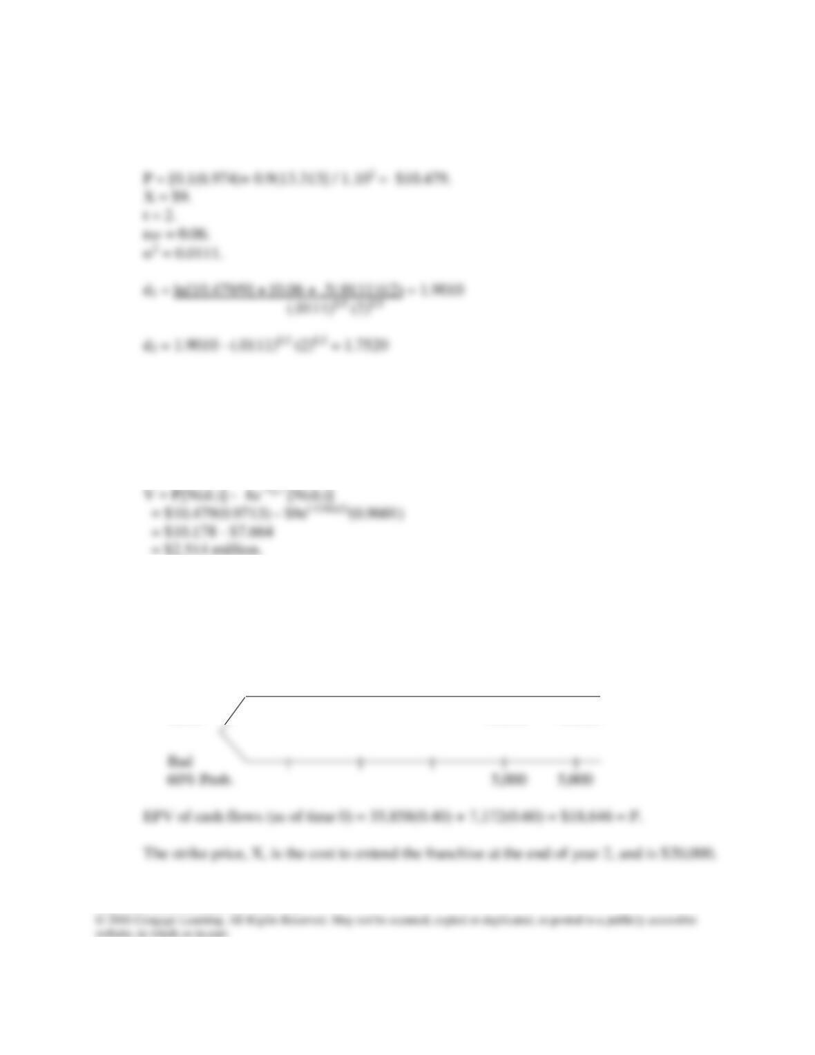
14-6 P = PV of all expected future cash flows if project is delayed. From Problem 14-1 we

know that PV @ Year 1 of Tax Imposed scenario is $15.45 and PV @ Year 1 of Tax Not

Imposed Scenario is $26.69. So the PV is:

From Excel function NORMSDIST, or approximated from the table in Appendix A:

N(d1) = 0.5670

N(d2) = 0.4628

Using the Black-Scholes Option Pricing Model, you calculate the option’s value as:

14-7 P = PV of all expected future cash flows if project is delayed. From Problem 14-1 we

know that PV @ Year 2 of Low CF Scenario is $6.974 and PV @ Year 2 of High CF

Scenario is $13.313. So the PV is:

From Excel function NORMSDIST, or approximated from the table in Appendix A:

N(d1) = 0.9713

N(d2) = 0.9601

Using the Black-Scholes Option Pricing Model, you calculate the option’s value as:

14-8 P = PV as of time zero of all expected future cash flows if the project is repeated starting

in year 2. Note it includes both the good cash flows and the bad cash flows since as of

now, we don’t know which outcome will result, and P excludes the $20,000 investment in

the franchise.

0 1 2 3 4

Good 25,000 25,000

r = 10%

Answers and Solutions: 14 – 12

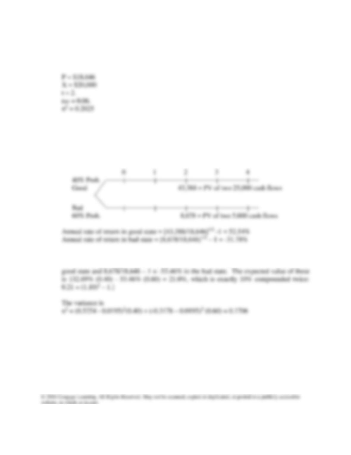
The time to expiration is the time you decide whether or not to extend the franchise, and is

at the end of year 2.

Although the problem stated to assume the variance of the project’s rate of return was

0.2025, we’ll also calculate it using the direct method. First calculate the rates of return

using the decision tree. To do this, calculate the present values of the two branches as of

the exercise date, year 2, and the rates of return assuming the initial value of the investment

was P = $18,646.

The expected value of these two returns is 52.54(0.40) – 31.78(0.60) = 1.95% [Note: this

isn’t 10% as you might hope! The 2-year returns are 43,388/18,646 – 1 = 132.69% in the

Answers and Solutions: 14 – 13

To calculate the variance of the project’s returns using the indirect method, first calculate

the standard deviation of the value at year 2. The value is either 43,388 (probability 40%)

or 8,678 (probability 60%).

Notice that in this case the direct method and the indirect method give very similar results

for σ.

P = $18,646

From Excel function NORMSDIST, or approximated from the table in Appendix A:

N(d1) = 0.6542

N(d2) = 0.4053

Using the Black-Scholes Option Pricing Model, you calculate the option’s value as:

Answers and Solutions: 14 – 14