
SOLUTION TO SPREADSHEET PROBLEMS
14-9 The detailed solution for the problem is available in the file, Ch 14 P9 Build a Model
Solution.xls, on the textbook’s Web site.
Answers and Solutions: 14 – 15

MINI CASE
Assume that you have just been hired as a financial analyst by Tropical Sweets Inc., a mid-
sized California company that specializes in creating exotic candies from tropical fruits such
as mangoes, papayas, and dates. The firm’s CEO, George Yamaguchi, recently returned
from an industry corporate executive conference in San Francisco, and one of the sessions
he attended was on real options. Since no one at Tropical Sweets is familiar with the basics
of real options, Yamaguchi has asked you to prepare a brief report that the firm’s executives
could use to gain at least a cursory understanding of the topics.
To begin, you gathered some outside materials the subject and used these materials to
draft a list of pertinent questions that need to be answered. In fact, one possible approach
to the paper is to use a question-and-answer format. Now that the questions have been
drafted, you have to develop the answers.
a. What are some types of real options?
Answer: 1. Investment timing options
2. Growth options
b. What are five possible procedures for analyzing a real option?
Answer: 1. DCF analysis of expected cash flows, ignoring option.
Mini Case: 14 – 16

c. Tropical Sweets is considering a project that will cost $70 million and will generate
expected cash flows of $30 per year for three years. The cost of capital for this
type of project is 10 percent and the risk–free rate is 6 percent. After discussions
with the marketing department, you learn that there is a 30 percent chance of high
demand, with future cash flows of $45 million per year. There is a 40 percent
chance of average demand, with cash flows of $30 million per year. If demand is
low (a 30 percent chance), cash flows will be only $15 million per year. What is
the expected NPV?
Answer: Initial Cost = $70 Million
Alternatively, one could calculate the NPV of each scenario:
Demand Probability Annual Cash Flow
High 30% $45
Find NPV of each scenario:
PV High: N=3 I=10 PV=? PMT=-45 FV=0
PV= 111.91
Mini Case: 14 – 17

d. Now suppose this project has an investment timing option, since it can be delayed
for a year. The cost will still be $70 million at the end of the year, and the cash
flows for the scenarios will still last three years. However, Tropical Sweets will
know the level of demand, and will implement the project only if it adds value to
the company. Perform a qualitative assessment of the investment timing option’s
value.
Answer: If we immediately proceed with the project, its expected NPV is $4.61 million.
However, the project is very risky. If demand is high, NPV will be $41.91 million.
Mini Case: 14 – 18

e. Use decision tree analysis to calculate the NPV of the project with the investment
timing option.
Answer: The project will be implemented only if demand is average or high.
Here is the time line:
0 1 2 3 4
High $0 -$70 $45 $45 $45
To find the NPVC, discount the cost at the risk-free rate of 6 percent since it is known
for certain, and discount the other risky cash flows at the 10 percent cost of capital.
f. Use a financial option pricing model to estimate the value of the investment timing
option.
Answer: The option to wait resembles a financial call option— we get to “buy” the project for
$70 million in one year if value of project in one year is greater than $70 million.
This is like a call option with a strike price of $70 million and an expiration date of
one year.
Mini Case: 14 – 19
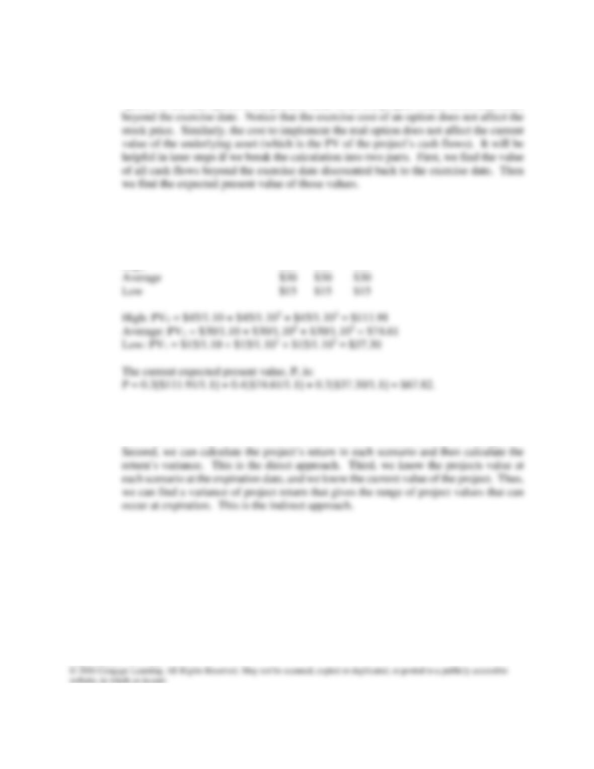
We explain how to calculate P and σ2 below.
Just as the price of a stock is the present value of all the stock’s future cash flows, the
“price” of the real option is the present value of all the project’s cash flows that occur
Step 1: Find the value of all cash flows beyond the exercise date discounted back to the
exercise date. Here is the time line. The exercise date is year 1, so we discount all
future cash flows back to year 1.
0 1 2 3 4
High $45 $45 $45
For a stock option, σ2 is the variance of the stock return, not the variance of the stock
price. Therefore, for a real option we need the variance of the project’s rate of return.
There are three ways to estimate this variance. First, we can use subjective judgment.
Mini Case: 14 – 20
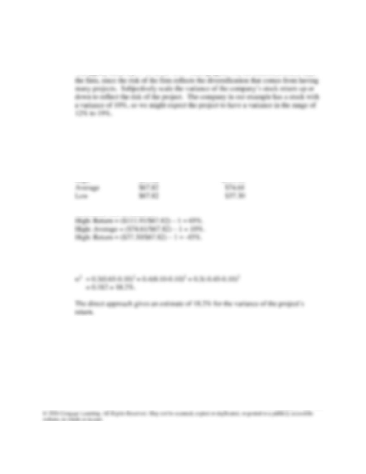
Following is an explanation of each approach.
Subjective estimate:
The typical stock has σ2 of about 12%. Most projects will be somewhat riskier than
Direct approach:
From our previous analysis, we know the current value of the project and the value
for each scenario at the time the option expires (year 1). Here is the time line:
Current Value Value At Expiration
Year 0 Year 1
The annual rate of return is:
Expected Return = 0.3(0.65) + 0.4(0.10) + 0.3(-0.45)
= 10%.
Mini Case: 14 – 21
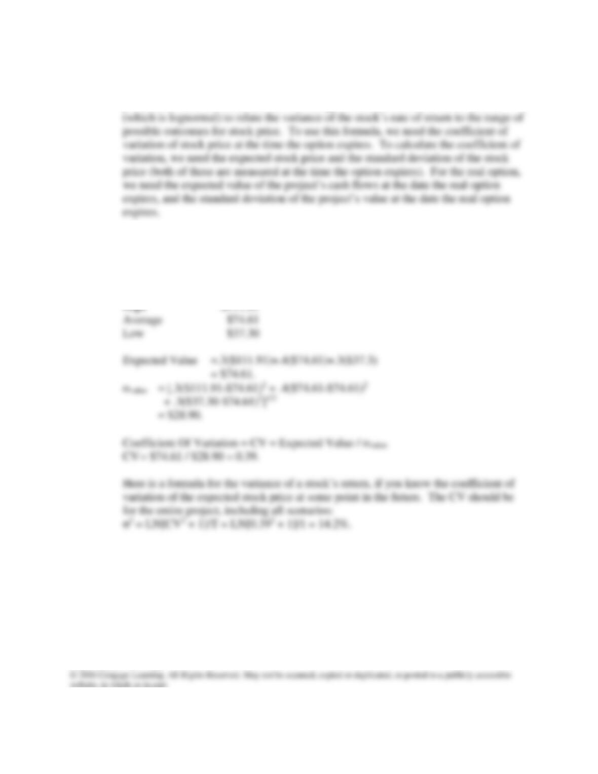
The indirect approach:
Given a current stock price and an anticipated range of possible stock prices at some
point in the future, we can use our knowledge of the distribution of stock returns
We previously calculated the value of the project at the time the option expires, and
we can use this to calculate the expected value and the standard deviation.
Value At Expiration
Year 1
Mini Case: 14 – 22

Now, we proceed to use the OPM:
g. Now suppose the cost of the project is $75 million and the project cannot be
delayed. But if Tropical Sweets implements the project, then Tropical Sweets will
have a growth option. It will have the opportunity to replicate the original project
at the end of its life. What is the total expected NPV of the two projects if both
are implemented?
Answer: Suppose the cost of the project is $75 million instead of $70 million, and there is no
option to wait.
NPV = PV of future cash flows – cost
Mini Case: 14 – 23
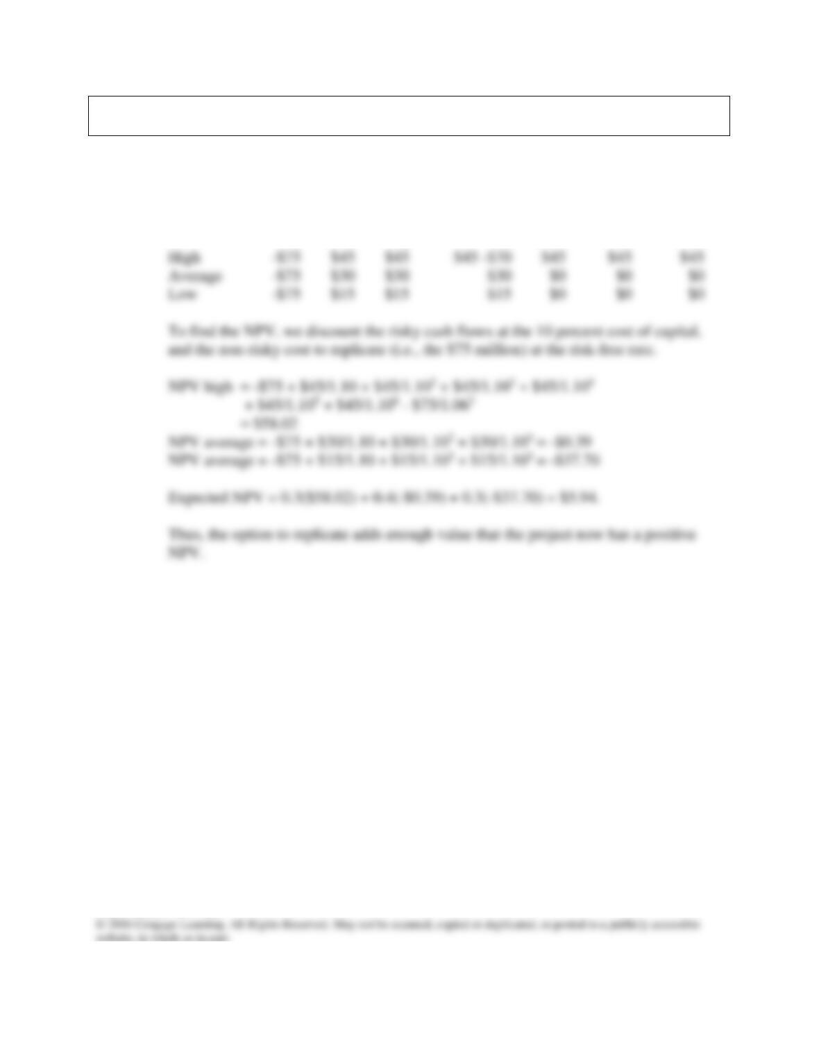
h. Tropical Sweets will replicate the original project only if demand is high. Using
decision tree analysis, estimate the value of the project with the growth option.
Answer: The future cash flows of the optimal decisions are shown below. The cash flow in year
3 for the high demand scenario is the cash flow from the original project and the cost
of the replication project.
0 1 2 3 4 5 6
Mini Case: 14 – 24

i. Use a financial option model to estimate the value of the growth option.
Answer: X = Strike Price = Cost Of Implement Project = $75 million.
σ2 = Variance Of Stock Return = Variance Of Project’s Rate Of Return.
We explain how to calculate P and σ2 below.
Step 1: Find the value of all cash flows beyond the exercise date discounted back to the
High: PV3 = $45/1.10 + $45/1.102 + $45/1.103 = $111.91
Mini Case: 14 – 25

Direct approach for estimating σ2:
From our previous analysis, we know the current value of the project and the value
for each scenario at the time the option expires (year 3). Here is the time line:
Current Value Value At Expiration
Year 0 Year 3
The annual rate of return is:
High: Return = ($111.91/$56.02)(1/3) – 1 = 25.9%.
This is lower than the variance found for the previous option because the dispersion
of cash flows for the replication project is the same as for the original, even though
the replication occurs much later. Therefore, the rate of return for the replication is
less volatile. We do sensitivity analysis later.

The indirect approach:
First, find the coefficient of variation for the value of the project at the time the option
expires (year 3).
We previously calculated the value of the project at the time the option expires, and
we can use this to calculate the expected value and the standard deviation.
Value At Expiration
Year 3
Coefficient of Variation = CV = Expected Value / σvalue
CV = $74.61 / $28.90 = 0.39.
Mini Case: 14 – 27

Now, we proceed to use the OPM:
Therefore,
V = $56.06(0.4568) – $75e–(0.06)(3)(0.3142)
= $5.92.
j. What happens to the value of the growth option if the variance of the project’s
return is 14.2 percent? What if it is 50 percent? How might this explain the high
valuations of many dot.com companies?
Answer: If risk, defined by σ2, goes up, then value of growth option goes up (see the file Ch14
mini case.xls for calculations):
Mini Case: 14 – 28