
1/1/2015
Chapter 13 Mini Case
Situation
Analysis of New Expansion Project
Part I: Input Data
Equipment cost $200,000 Key Output: NPV = $88,010
Shipping charge $10,000
Installation charge $30,000
Annual Depreciation Expense
Depreciable Basis = Equipment + Freight + Installation
Depreciable Basis = $240,000
Year % x Basis = Depr.
Remainin
g Book
Value
1 0.3333 $240,000 $79,992 $160,008
Shrieves Casting Company is considering adding a new line to its product mix, and the capital budgeting
analysis is being conducted by Sidney Johnson, a recently graduated MBA. The production line would be set
up in unused space in Shrieves’ main plant. The machinery’s invoice price would be approximately $200,000,
another $10,000 in shipping charges would be required, and it would cost an additional $30,000 to install the
equipment. The machinery has an economic life of 4 years, and Shrieves has obtained a special tax ruling that
places the equipment in the MACRS 3-year class. The machinery is expected to have a salvage value of
$25,000 after 4 years of use.
The new line would generate incremental sales of 1,250 units per year for 4 years at an incremental cost of
$100 per unit in the first year, excluding depreciation. Each unit can be sold for $200 in the first year. The
sales price and cost are expected to increase by 3% per year due to inflation. Further, to handle the new line,
the firm’s net working capital would have to increase by an amount equal to 12% of sales revenues. The firm’s
tax rate is 40%, and its overall weighted average cost of capital is 10%.
included in the analysis? Explain. Answer: See Chapter 13 Mini Case Show
be included in the analysis? If so, how? Answer: See Chapter 13 Mini Case Show
(3.) Now assume that the plant space could be leased out to another firm at $25,000 per year. Should this
(4.) Finally, assume that the new product line is expected to decrease sales of the firm’s other lines by
b. Disregard the assumptions in Part a. What is Shrieves’ depreciable basis? What are the annual
depreciation expenses?
Economic Life 4
Salvage Value $25,000
Tax Rate 40%
Cost of Capital 10%
Units Sold 1,250
Sales Price Per Unit $200
Incremental Cost Per Unit $100
Inflation rate 3%
Annual Operating Cash Flows
Year 1 Year 2 Year 3 Year 4
Units 1,250 1,250 1,250 1,250
Unit price $200.00 $206.00 $212.18 $218.55
Unit cost $100.00 $103.00 $106.09 $109.27
Depreciation 79,992 106,680 35,544 17,784
Operating income before taxes (EBIT) $45,008 $22,070 $97,069 $118,807
Depreciation 79,992 106,680 35,544 17,784
Annual Cash Flows due to Investments in Net Working Capital
Year 0 Year 1 Year 2 Year 3 Year 4
NWC (% of sales) 30,000 30,900 31,827 32,782
CF due to investment in NOWC) (30,000) (900) (927) (955) 32,782
d. Construct annual incremental operating cash flow statements.
e. Estimate the required net working capital for each year, and the cash flow due to investments in net
working capital.
c. Calculate the annual sales revenues and costs (other than depreciation). Why is it important to include

f. Calculate the after-tax salvage cash flow.
After-tax Salvage Value
Based on
facts in
case:
$25,000 $10,000
Projected Net Cash Flows
Year 0 Year 1 Year 2 Year 3 Year 4
Net Cash Flows ($270,000) $106,097 $118,995 $92,830 $136,850
NPV $88,010
IRR 23.9%
PV of Inflows
TV of Inflows
$358,010 $524,162
Find MIRR 0 1 2 3 4
MIRR = 18.0%
Find Payback
0 1 2 3 4
Hypothetical: If sold
after 3 years for
Years
g. Calculate the net cash flows for each year. Based on these cash flows, what are the project’s NPV, IRR,
MIRR, and payback? Do these indicators suggest the project should be undertaken?
Years
To find MIRR, we could now find the discount rate that equates the PV and TV. But it is easier to use the MIRR
function.
Net terminal cash flow $15,000 $22,114 $13,114

Evaluating Risk: Sensitivity Analysis
Sensitivity of NPV and to Variations in Input Variables
% Deviation % Deviation
% Deviation
from NPV from Units NPV from Variable NPV
Base Case WACC 88,010 Base Case Sold $88,010 Base Case Cost $88,010
i. (1.) What are the three types of risk that are relevant in capital budgeting? Answer: See Chapter 13 Mini
(3.) How is each type of risk used in the capital budgeting process? Answer: See Chapter 13 Mini Case
(2.) Perform a sensitivity analysis on the unit sales, salvage value, and cost of capital for the project.
Assume that each of these variables can vary from its base-case, or expected, value by plus and minus 10%,
20%, and 30%. Include a sensitivity diagram, and discuss the results.
(2.) How is each of these risk types measured, and how do they relate to one another? Answer: See
h. What does the term ”risk” mean in the context of capital budgeting; to what extent can risk be quantified;
and when risk is quantified, is the quantification based primarily on statistical analysis of historical data or on
subjective, judgmental estimates?
Risk in capital budgeting really means the probability that the actual outcome will be worse than the expected
outcome. For example, if there were a high probability that the expected NPV as calculated above will actually
turn out to be negative, then the project would be classified as relatively risky. The reason for a worse-than-
expected outcome is, typically, because sales were lower than expected, costs were higher than expected,
and/or the project turned out to have a higher than expected initial cost. In other words, if the assumed inputs
turn out to be worse than expected then the output will likewise be worse than expected. We use Excel to
examine the project’s sensitivity to changes in the input variables.
WACC
Here we use an Excel “Data Table” to find the NPVs for changes in unit sales, salvage value, and WACC
We summarize the data tables and show the sensitivity analysis graph below:
1st YEAR UNIT SALES
SALVAGE
j. (1.) What is sensitivity analysis? Answer: See Chapter 13 Mini Case Show
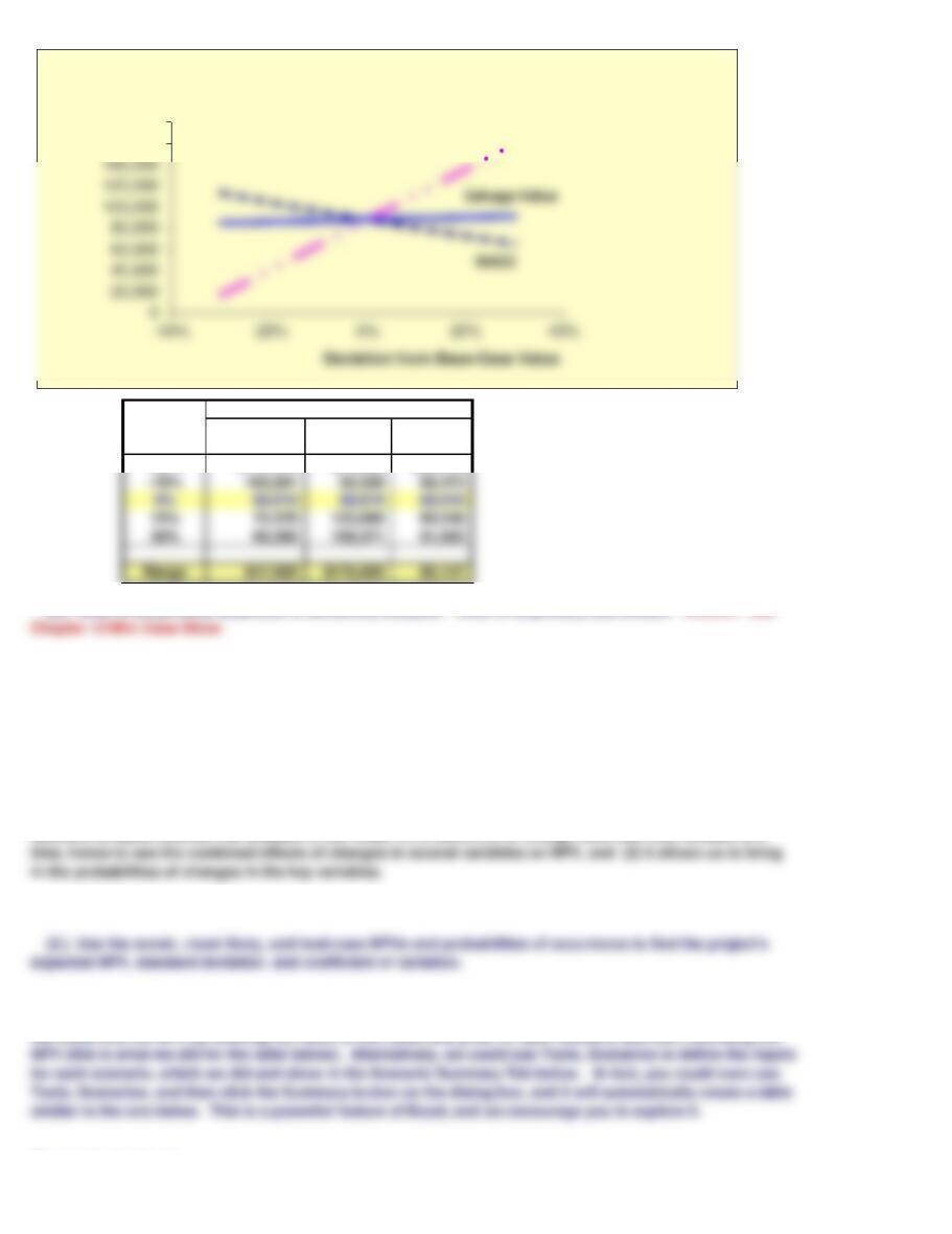
Evaluating Risk: Sensitivity Analysis
Deviation NPV Deviation from Base Case
from Units
Base Case WACC Sold Salvage
-30% $113,270 $16,649 $84,936
Evaluating Risk: Scenario Analysis
Scenario Analysis
(3.) What is the primary weakness of sensitivity analysis? What is its primary usefulness? Answer: See
We could find the NPV by entering the value of unit sales and price for each scenario and then recording the
k. Assume that Sidney Johnson is confident of her estimates of all the variables that affect the project’s cash
flows except unit sales and sales price: If product acceptance is poor, unit sales would be only 900 units a
year and the unit price would only be $160; a strong consumer response would produce sales of 1,600 units
and a unit price of $240. Sidney believes that there is a 25% chance of poor acceptance, a 25% chance of
excellent acceptance, and a 50% chance of average acceptance (the base case).
(1.) What is scenario analysis?
(2.) What is the worst-case NPV? The best-case NPV?
expected NPV, standard deviation, and coefficient of variation.
Squared Deviation
Scenario analysis extends risk analysis in two ways: (1) It allows us to change more than one variable at a
160,000
180,000
NPV ($)
Sensitivity Analysis
Units Sold

Probability Unit Sales Unit Price NPV
25% 1,600 $240 $278,940
Monte Carlo Simulation
Risk Adjusted Cost of Capital
(2.) Shrieves typically adds or subtracts 3 percentage points to the overall cost of capital to adjust for risk.
Should the new line be accepted?
(3.) Are there any subjective risk factors that should be considered before the final decision is made?
times Probability
n. What is a real option? What are some types of real options? Answer: See Chapter 13 Mini Case Show
The CV of this project is 1.15, which is larger than the CV range of the firm’s average project. Consequently,
this project is riskier than the firm’s average project, so management should add 3% to the WACC to risk
$7,861,657,811.87
m. (1.) Assume that Shrieves’ average project has a coefficient of variation in the range of 0.2 to 0.4. Would
the new line be classified as high risk, average risk, or low risk? What type of risk is being measured here?
Best Case
Monte Carlo simulation is similar to scenario analysis in that different values of key input variables are used.
Scenario
l. Are there problems with scenario analysis? Define simulation analysis, and discuss its principal
50% 1,250 $200 $88,010
$5,635,163,606.11
Scenario Summary
Current Values: Base Case Best Case Worst Case Base-but forget inflation
Changing Cells:
$D$36 $200,000 $200,000 $200,000 $200,000 $200,000
$D$37 $10,000 $10,000 $10,000 $10,000 $10,000
$D$38 $30,000 $30,000 $30,000 $30,000 $30,000
Result Cells:
1/1/2015
Analysis of New Expansion Project
Part I: Input Data
Equipment cost $200,000 Key Output: NPV = $75,326
Shipping charge $10,000
Installation charge $30,000
Annual Depreciation Expense
Depreciable Basis = Equipment + Freight + Installation
Depreciable Basis = $240,000
Annual Operating Cash Flows
Year 1 Year 2 Year 3 Year 4
Units 841 841 841 841
Unit price $239.80 $247.00 $254.41 $262.04
Unit cost $100.00 $103.00 $106.09 $109.27
Depreciation 79,200 108,000 36,000 16,800
Operating income before taxes (EBIT) $38,426 $13,155 $88,794 $111,739
Taxes (40%) 15,370 5,262 35,518 44,696
Depreciation 79,200 108,000 36,000 16,800
Section 13.7 Scenario Analysis
Monte Carlo simulation is similar to scenario analysis in that different values of key inputs are used Unlike scenario
analysis, Monte Carlo simulation draws a trial set of input values from specified probability distributions and then
computes the NPV for this trial. This process is repeated for hundreds, or even thousands, of trials, with key results (like
NPV) saved from each trial. After running the number of desired trials, the NPVs from the trials can be averaged to estimate
the project’s expected NPV; the trial results can also be used to provide a histogram showing the project’s possible
outcomes.
inflation when estimating cash flows? See answer to part d.
b. Disregard the assumptions in Part a. What is Shrieves’ depreciable basis? What are the annual
d. Construct annual incremental operating cash flow statements.
Economic Life 4
Salvage Value $25,000
Tax Rate 40%
Units Sold Random variable = 841 1,250 200
Sales Price Per Unit Random variable = $240 $200 $30
Incremental Cost Per Unit $100
Inflation rate 3%
Annual Cash Flows due to Investments in Net Working Capital
f. Calculate the after-tax salvage cash flow.
After-tax Salvage Value
Based on
facts in
case:
$25,000 $10,000
Net terminal cash flow $15,000 $21,720 $12,720
Projected Net Cash Flows
Year 0 Year 1 Year 2 Year 3 Year 4
Net Cash Flows ($264,212) $101,530 $115,144 $88,506 $125,300
NPV $75,326
IRR 22.3%
PV of Inflows
TV of Inflows
$339,538 $497,118
Find MIRR 0 1 2 3 4
MIRR = 17.1%
Find Payback
How the Simulation Works
e. Estimate the required net working capital for each year, and the cash flow due to investments in net working
capital.
To find MIRR, we could now find the discount rate that equates the PV and TV. But it is easier to use the MIRR function.
Excel normally updates all values in a Data Table each time any cell that is related to the Data Table changes. In our case,
we have random variables in the Data Table, so each time any cell in the worksheet makes a calculation, the Data Table is
updated. If the Data Table has many rows, updating it can take up to 20 or 30 seconds. With only 100 rows, it updates very
quickly. But if it bothers you, you can set the worksheet to do automatic calculation except for data tables.
Hypothetical: If sold
g. Calculate the net cash flows for each year. Based on these cash flows, what are the project’s NPV, IRR,
MIRR, and payback? Do these indicators suggest the project should be undertaken?
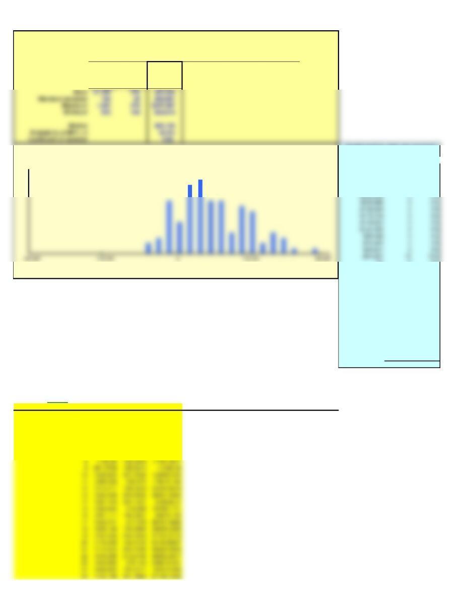
We use a Data Table to perform the simulation (the Data Table is below, shaded bright yellow). When the Data Table is
updated, it will insert new random variables for each of the inputs we allow to change in Panel A above, run the analysis is
Panel C above, and then save the NPV for each trial (we also save the input variables for each trial so that we can verify that
they are behaving as we expect). We set the first column of the Data Table (the variable to be changed in each row) to
numbers from 1-100. We don‘t really use these numbers anywhere in the analyis, but if we tell the Data Table to treat these
Years
Years
Number of Trials = 100
NPV
Scratch work for chart: see comments.
Count
Range bottom 0Percent
-$347,487 0 0%
-$322,667 0 0%
-$297,846 0 0%
-$273,026 0 0%
$0 66%
$24,821 13 13%
$49,641 14 14%
$74,462 10 10%
$99,282 10 10%
$124,103 44%
$148,923 99%
$173,744 88%
$198,564 22%
$223,385 44%
$248,205 33%
$273,026 11%
$297,846 00%
$322,667 11%
$347,487 00%
Sum 100 100%
Output of Simulation in Data Table
Trial Number Units Sold
Sales
Price Per
Unit
NPV
841 $240 $75,326
11482.162 179.6793 73697.4367
21450.372 278.5524 347487.078
31636.094 208.8927 189759.009
41292.922 206.0437 111373.894
51525.659 208.3979 165373.307
61089.843 226.0634 112727.776
71238.148 208.9191 107223.129
Figure 13-7 Summary of Simulation Results (Thousands of Dollars)
Units Sold
Sales
Price Per
Unit
Simulated Input Variables and Key Results
Key
Results:
Probability
NPV ($)

26 1181.457 157.7572 -21972.4905
27 1375.427 202.0806 117457.616
28 1373.72 187.9796 79494.9509
29 1681.014 236.7247 289970.897
30 1218.892 164.7006 -1476.39929
31 868.0948 159.6303 -52727.3457
40 1251.711 220.6765 138633.239
41 1252.044 181.556 43554.7336
42 1312.242 216.6936 142427.913
43 1224.086 183.961 44950.5073
44 1374.824 189.8644 84713.8238
45 1382.347 149.0617 -23576.1831
46 1254.626 183.8015 49433.853
47 1322.338 209.3552 125817.219
48 1061.469 196.253 44421.6458
62 1486.626 191.7699 109288.305
63 1393.849 177.2979 53934.9915
64 1302.656 212.8391 130534.434
65 1410.309 181.3553 67452.4482
66 1582.962 216.8509 203210.496
67 1459.516 240.8791 243804.669
68 995.7285 200.453 40516.7101
69 1278.886 174.0809 29129.7247
81 1299.772 194.9364 84713.4725
82 1290.756 188.7481 67568.4999
83 1346.455 182.5186 60653.9732
84 1203.858 232.1267 154377.236
85 956.1948 157.9672 -45955.6129
86 1362.29 227.9354 183326.018
87 1427.823 214.5954 162344.503
88 1078.102 247.8192 155464.783
89 1229.56 166.1606 3311.87433