CFIN6 – CHAPTER 12
INTEGRATIVE PROBLEM SOLUTION
a(1). Business risk is the uncertainty associated with a firm’s projection of its future operating income. It also
is defined as the risk faced by a firm’s stockholders if the company uses no debt. A firm’s business risk
(6) special risk factors (such as potential product liability for a drug company or the potential cost of a
nuclear accident for a utility with nuclear plants).
a(2). Operating leverage is the extent to which fixed operating costs are used in a firm’s operations. If a high
percentage of the firm’s total operating costs are fixed, and hence do not decline when demand falls,
then the firm is said to have high operating leverage. Other things held constant, the greater a firm’s
operating leverage, the greater its business risk.
b(1). Financial leverage refers to the firm’s decision to finance with fixed-charge securities, such as debt and
b(2). As we discussed above, business risk depends on a number of factors such as sales and cost
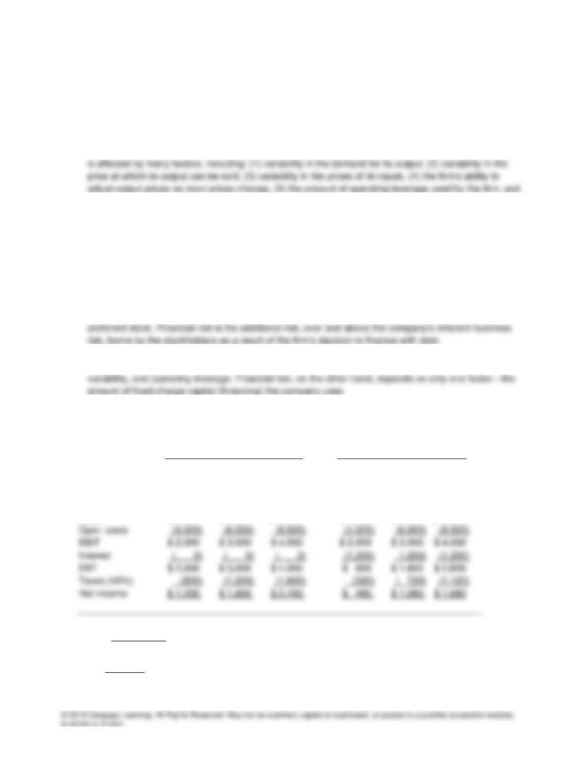
c(1). Here are the fully completed statements:
Firm U Firm L
Assets $20,000 $20,000 $20,000 $20,000 $20,000 $20,000
Equity $20,000 $20,000 $20,000 $10,000 $10,000 $10,000
Probability 0.25 0.50 0.25 0.25 0.50 0.25
Sales $ 6,000 $ 9,000 $12,000 $ 6,000 $ 9,000 $12,000
ROE
equity Common
income Net
=
6.0% 9.0% 12.0% 4.8% 10.8% 16.8%
TIE
income Net
EBIT
=
∞ ∞ ∞ 1.7x 2.5x 3.3x
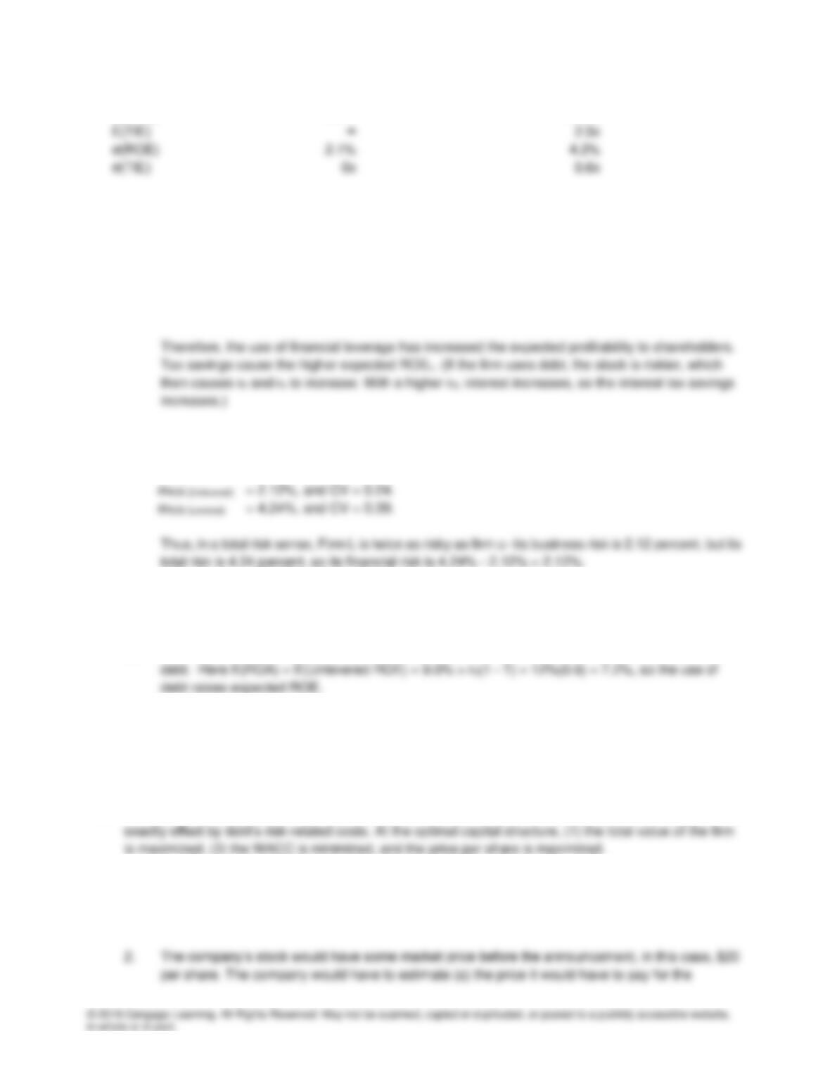
E(ROE) 9.0% 10.8%
c(2). Conclusions from the analysis:
(1) Firm L has the higher expected ROE:
E(ROEU) = 0.25(6.0%) + 0.50(9.0%) + 0.25(12.0%) = 9.0%
E(ROEL) = 0.25(4.8%) + 0.50(10.8%) + 0.25(16.8%) = 10.8%
(2) Firm L has a wider range of ROEs, and a higher standard deviation of ROE, indicating that its
higher expected return is accompanied by higher risk. To be precise:
(3) When EBIT = $2,000, ROEU > ROEL, and leverage has a negative impact on profitability.
However, at the expected level of EBIT, ROEL > ROEU.
(4) Leverage will boost expected ROE if the expected unlevered ROA exceeds the after-tax cost of
(5) Finally, note that the TIE ratio is huge (undefined, or infinitely large) if no debt is used, but it is
relatively low if 50 percent debt is used. The expected TIE would be larger than 2.5x if less debt
were used, but smaller if leverage were increased.
d(1). The optimal capital structure is the capital structure at which the tax-related benefits of leverage are
d(2). Here is the sequence of events:
1. CDSS must first announce its recapitalization plans.
repurchased shares and (b) the method to be used for the repurchase (open market purchases,
or a tender offer).
3. For simplicity, we assume that the firm could repurchase stock at its current price, $20, which
also happens to be its book value per share. In actuality, investors would probably reassess their
4. CDSS would purchase stock, then issue debt and use the proceeds to pay for the repurchased
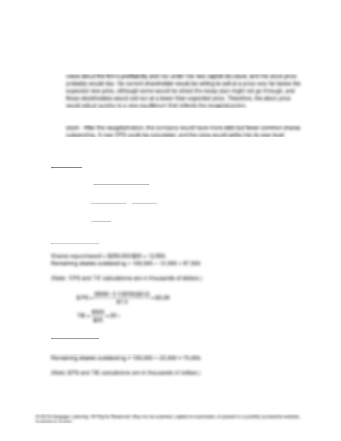
d(3). The analysis for the debt levels being considered (in thousands of dollars and shares) is shown below:
At Debt = $0:
=
nterestI
EBIT
= TIE
$3.00 =
100,000
$300,000
=
100,000
.6)$500,000(0
=
dingtanouts haresS
T) – )](1ebt(D
r
– [EBIT
= EPS d
At Debt = $250,000:
At Debt = $500,000:
Shares repurchased = $500,000/$20 = 25,000.

$3.56 =
75
](0.6)0.11($500) – [$500
= EPS
5.1 =
$97.5
$500
= TIE
$3.86 =
62.5
](0.6)0.13($750) – [$500
= EPS
At Debt = $1,000,000:
Shares repurchased = $1,000,000/$20 = 50,000.
Remaining shares outstanding = 100,000 ─ 50,000 = 50,000.
(Note: EPS and TIE calculations are in thousands of dollars.)
d(4). We can calculate the price of a constant growth stock as DPS divided by rs minus g, where g is the
expected growth rate in dividends:
g –
r
D
ˆ
=
Ps
1
0
Because in this case all earnings are paid out to the stockholders, DPS = EPS. Further, because no
earnings are plowed back, the firm’s EBIT is not expected to grow, so g = 0. Here are the results:
Debt Level DPS rs Stock Price
$ 0 $3.00 15.0% $20.00
d(5). A capital structure with $500,000 of debt produces the highest stock price, $21.58, hence it is the best
of those considered.
d(6). We have seen that EPS continues to increase beyond the $500,000 optimal level of debt. Therefore,
d(7). Currently, Debt/Total assets = 0%, so total assets = initial equity = $20 x 100,000 shares = $2,000,000.
WACC = ($500,000/$2,000,000)[(11%)(0.60)] + ($1,500,000/$2,000,000)(16.5%)
= 1.65% + 12.38% = 14.03%.
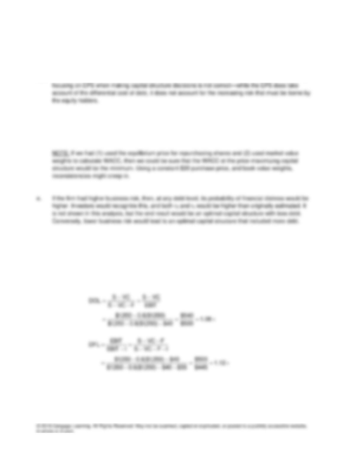
f. The three degrees of leverage are calculated below:
S = $1,350,000 New debt = $500,000 @ 11%
VC = 0.6 × S F = $40,000
(Note: Calculations are in thousands of dollars.)
DTL = DOL x DFL = 1.08 x 1.12 = 1.21.
The degree of operating leverage is defined as the percentage change in operating income (EBIT)
associated with a given percentage change in sales. Because our company’s degree of operating
leverage is 1.08, this means that a given percentage increase in sales will lead to an 8 percent greater
increase in EBIT. For example, if sales increased by 100 percent, then EBIT would increase by 108
percent.
they expect sales to rise or fall.
g. Because it is difficult to quantify the capital structure decision, managers consider the following judgmental
factors when making capital structure decisions:
(1) The average debt ratio for firms in their industry.
(2) Pro forma tie ratios at different capital structures under different scenarios.
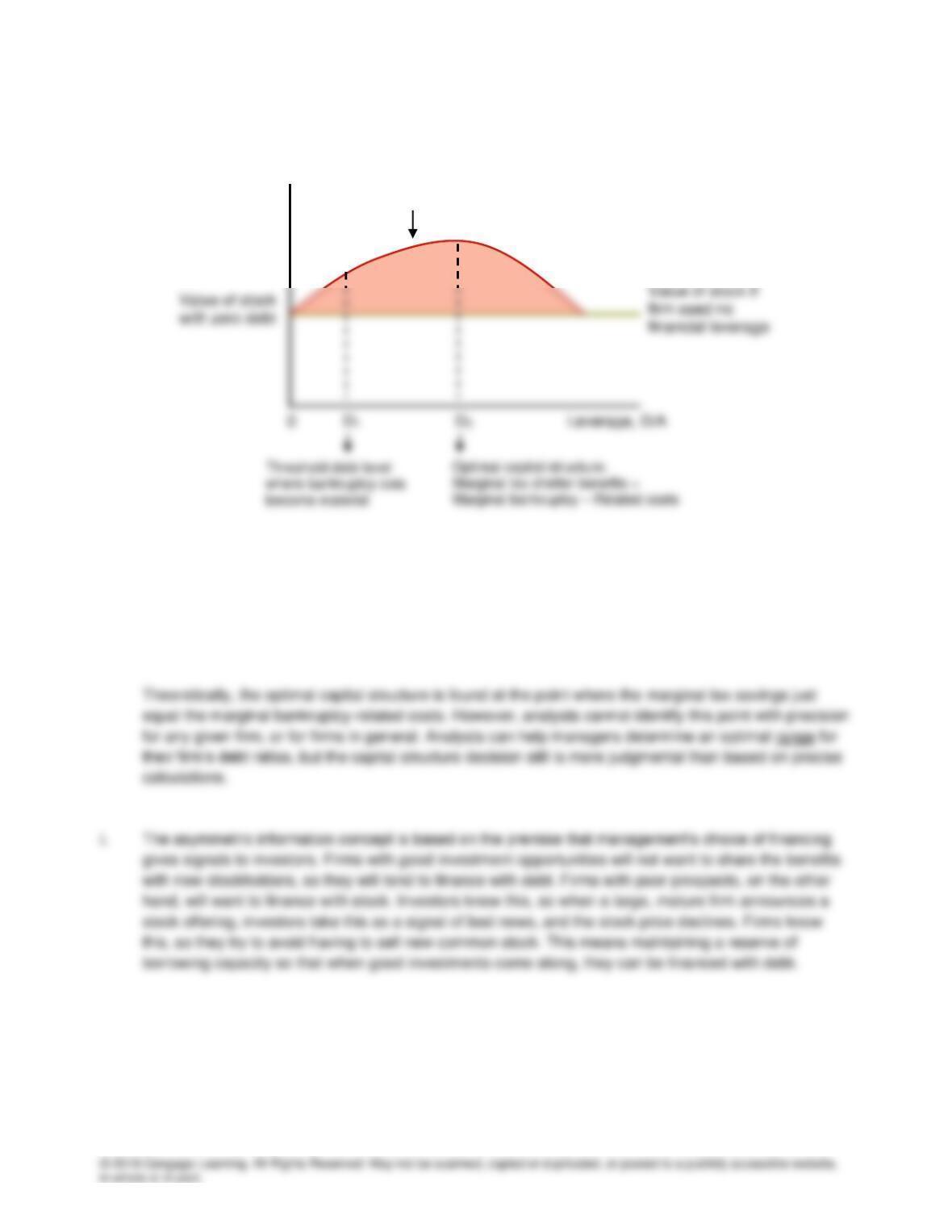
h. The following figure presents a graph of the situation:
The use of debt permits a firm to obtain tax savings from the deductibility of interest. So the use of
some debt is good; however, the possibility of bankruptcy increases the cost of using debt. At higher
and higher levels of debt, the risk of bankruptcy increases, bringing with it costs associated with
potential financial distress. Customers reduce purchases, key employees leave, and so on. There is
some point, generally well below a debt ratio of 100 percent, at which problems associated with
potential bankruptcy more than offset the tax savings from debt.
Value of
Firm’s Stock
Actual price
of stock