11/21/2018
Chapter 11 Mini Case
Situation
Part I: Input Data
Scenario: Base Case
Equipment cost $200,000 Key Outputs: NPV = $62,593
Shipping charge $10,000 IRR = 20.1%
Installation charge $30,000 MIRR = 16.0%
Economic Life 4PI = 1.24
Salvage Value $25,000 Payback = 2.76
Tax Rate 25% Discounted Payback = 3.30
Cost of Capital 10%
Units Sold 1,000
Sales Price Per Unit $200
Incremental Cost Per Unit $100
Inflation rate 3%
Annual Depreciation Expense
Depreciable Basis = Equipment + Freight + Installation
Depreciable Basis = $240,000
Year 1 Year 2 Year 3 Year 4
Basis $240,000
Depreciation rate 0.3333 0.4445 0.1481 0.0741
Depreciation expense $79,992.00 $106,680.00 $35,544.00 $17,784.00
Remaining book value $160,008.00 $53,328.00 $17,784.00 $0.00
Shrieves Casting Company is considering adding a new line to its product mix, and the capital budgeting analysis is being conducted by
Sidney Johnson, a recently graduated MBA. The production line would be set up in unused space in Shrieves‘ main plant. The machinery’s
invoice price would be approximately $200,000, another $10,000 in shipping charges would be required, and it would cost an additional
$30,000 to install the equipment. The machinery has an economic life of 4 years, and Shrieves has obtained a special tax ruling that places
the equipment in the MACRS 3-year class. The machinery is expected to have a salvage value of $25,000 after 4 years of use.
average project (r), is 10%.
a. Define “incremental cash flow.” Answer: See Chapter 11 Mini Case Show
Explain. Answer: See Chapter 11 Mini Case Show
(1.) Should you subtract interest expense or dividends when calculating project cash flow? Answer: See Chapter 11 Mini Case Show
If so, how? Answer: See Chapter 11 Mini Case Show
(4.) Finally, assume that the new product line is expected to decrease sales of the firm’s other lines by $50,000 per year. Should this be
considered in the analysis? If so, how? Answer: See Chapter 11 Mini Case Show
b. Disregard the assumptions in Part a. What is Shrieves‘ depreciable basis? What are the annual
depreciation expenses?
c. Calculate the annual sales revenues and costs (other than depreciation). Why is it important to include inflation when estimating cash
flows? See answer to part d.
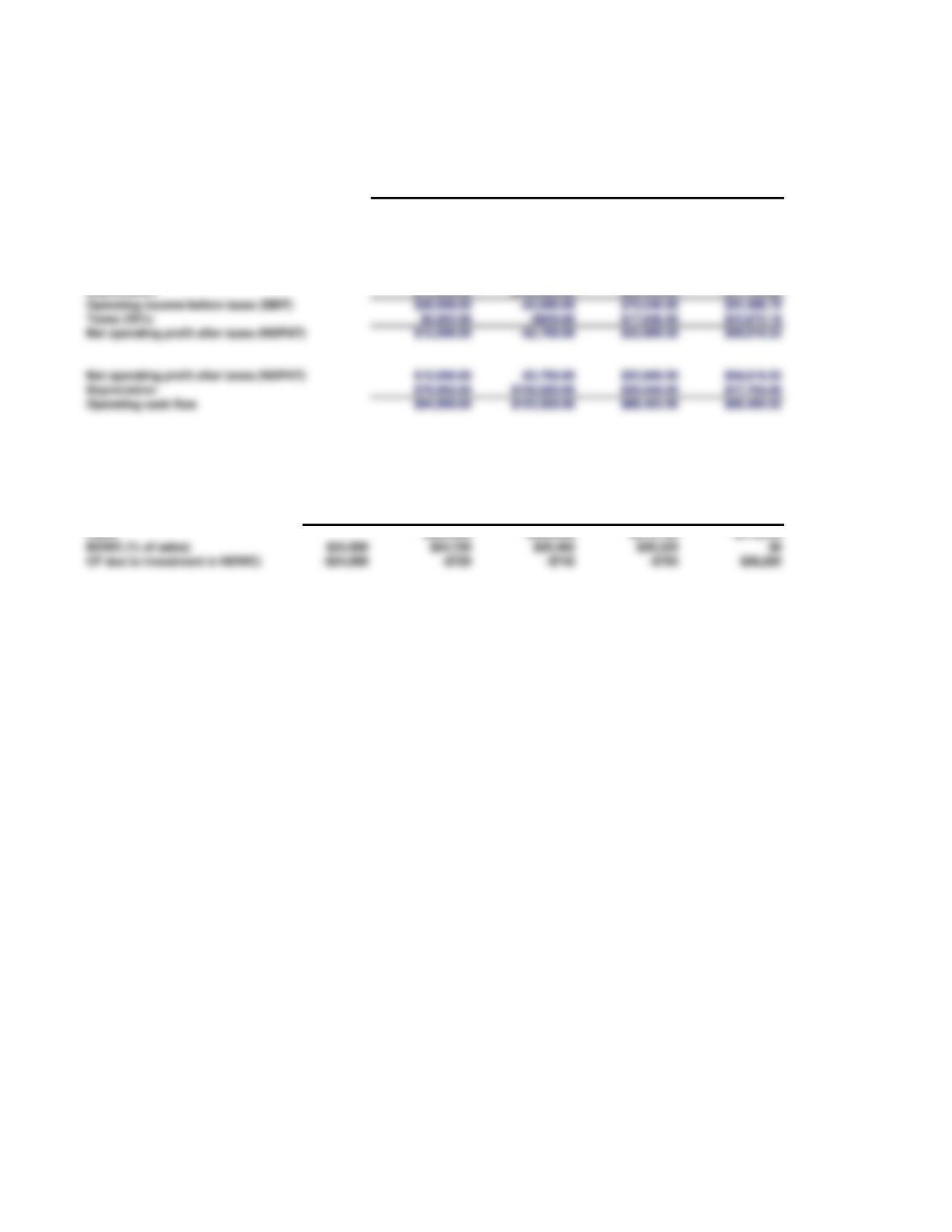
Annual Operating Cash Flows
Year 1 Year 2 Year 3 Year 4
Units 1,000 1,000 1,000 1,000
Unit price $200.00 $206.00 $212.18 $218.55
Unit cost $100.00 $103.00 $106.09 $109.27
Sales $200,000.00 $206,000.00 $212,180.00 $218,545.40
Costs $100,000.00 $103,000.00 $106,090.00 $109,272.70
Depreciation $79,992.00 $106,680.00 $35,544.00 $17,784.00
Operating income before taxes (EBIT) $20,008.00 -$3,680.00 $70,546.00 $91,488.70
Taxes (25%) $5,002.00 -$920.00 $17,636.50 $22,872.18
Net operating profit after taxes (NOPAT) $15,006.00 -$2,760.00 $52,909.50 $68,616.53
Net operating profit after taxes (NOPAT) $15,006.00 -$2,760.00 $52,909.50 $68,616.53
Operating cash flow $94,998.00 $103,920.00 $88,453.50 $86,400.53
Annual Cash Flows due to Investments in Net Working Capital
Year 0 Year 1 Year 2 Year 3 Year 4
NOWC (% of sales) $24,000 $24,720 $25,462 $26,225 $0
CF due to investment in NOWC) -$24,000 -$720 -$742 -$763 $26,225
d. Calculate annual net operating profit after sales (NOPAT).
e. Estimate the required net operating working capital (NOWC) for each year, and the cash flow due to investments in net working capital.
c. Calculate the annual sales revenues and costs (other than depreciation). Why is it important to include inflation when estimating cash
flows? See answer to part d.
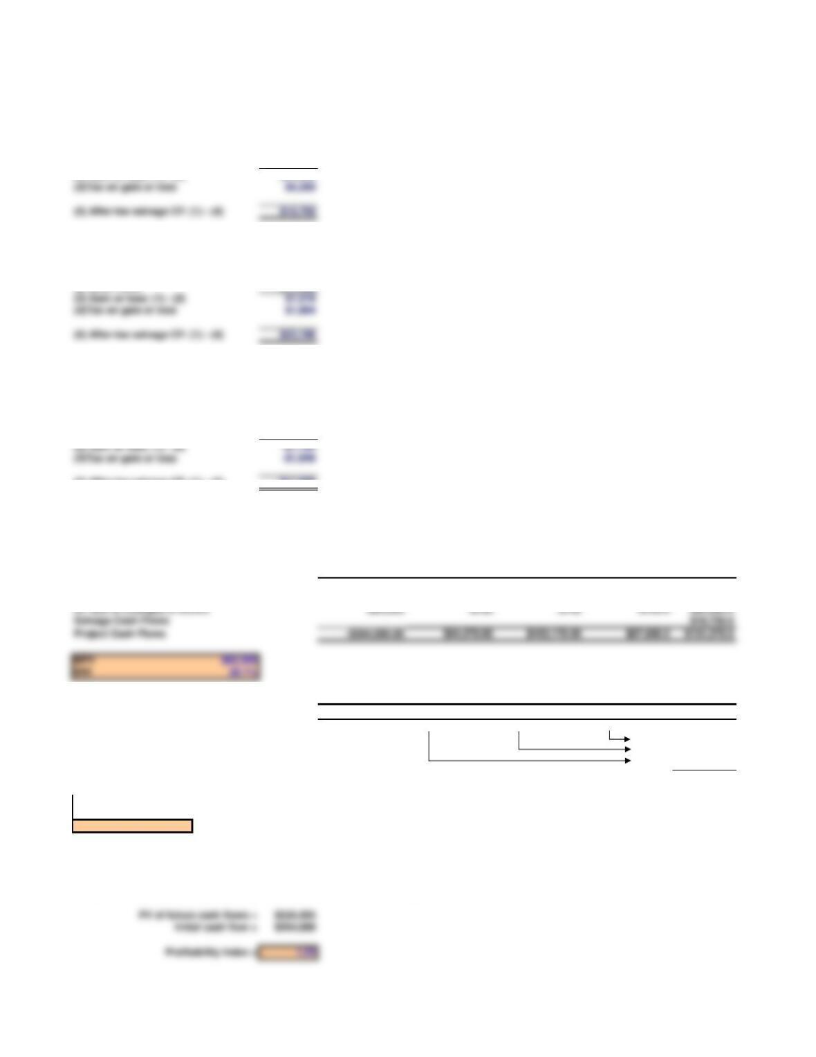
f. Calculate the after-tax salvage cash flow.
After-tax Salvage Value
(1) Salvage value $25,000
(2) Book value $0
(3) Gain or loss: (1) – (2) $25,000
(4)Tax on gain or loss $6,250
(5) After-tax salvage CF: (1) – (4) $18,750
If the project lasts only 3 years and the salvage value is $25,000, what is the after-tax salvage cash flow?
(1) Salvage value $25,000
(2) Book value $17,784
(3) Gain or loss: (1) – (2) $7,216
(4)Tax on gain or loss $1,804
(5) After-tax salvage CF: (1) – (4) $23,196
If the project lasts 3 year and the salvage value is $10,000, what is the after-tax salvage cash flow?
(1) Salvage value $10,000
(2) Book value $17,784
(3) Gain or loss: (1) – (2) -$7,784
(4)Tax on gain or loss -$1,946
(5) After-tax salvage CF: (1) – (4) $11,946
Operating Cash Flows
Year 0 Year 1 Year 2 Year 3 Year 4
Initial Cost -$240,000
Operating Cash Flows $94,998 $103,920 $88,453.5 $86,400.5
CF due to Changes in NOWC -$24,000 -$720 -$742 -$763.0 $26,225.0
Salvage Cash Flows $18,750.0
Project Cash Flows -$264,000.00 $94,278.00 $103,178.00 $87,690.5 $131,375.5
Find MIRR 0 1 2 3 4
Net Cash Flows -264,000 94,278 103,178 87,690.5 131,375.5
96,459.6
124,845.4
125,484.0
PV= -264,000 TV = 478,164.5
MIRR = 16.0%
Find the Profitability Index (PI)
The profitability index is the present value of future cash flows divided by initial cost.
g. Calculate the net cash flows for each year. Based on these cash flows and the average project cost of capital, what are the project’s NPV,
IRR, MIRR, PI, payback, and discounted payback? Do these indicators suggest that the project should be undertaken?
Years
To find MIRR, we could now find the discount rate that equates the PV and TV. But it is easier to use the MIRR function.
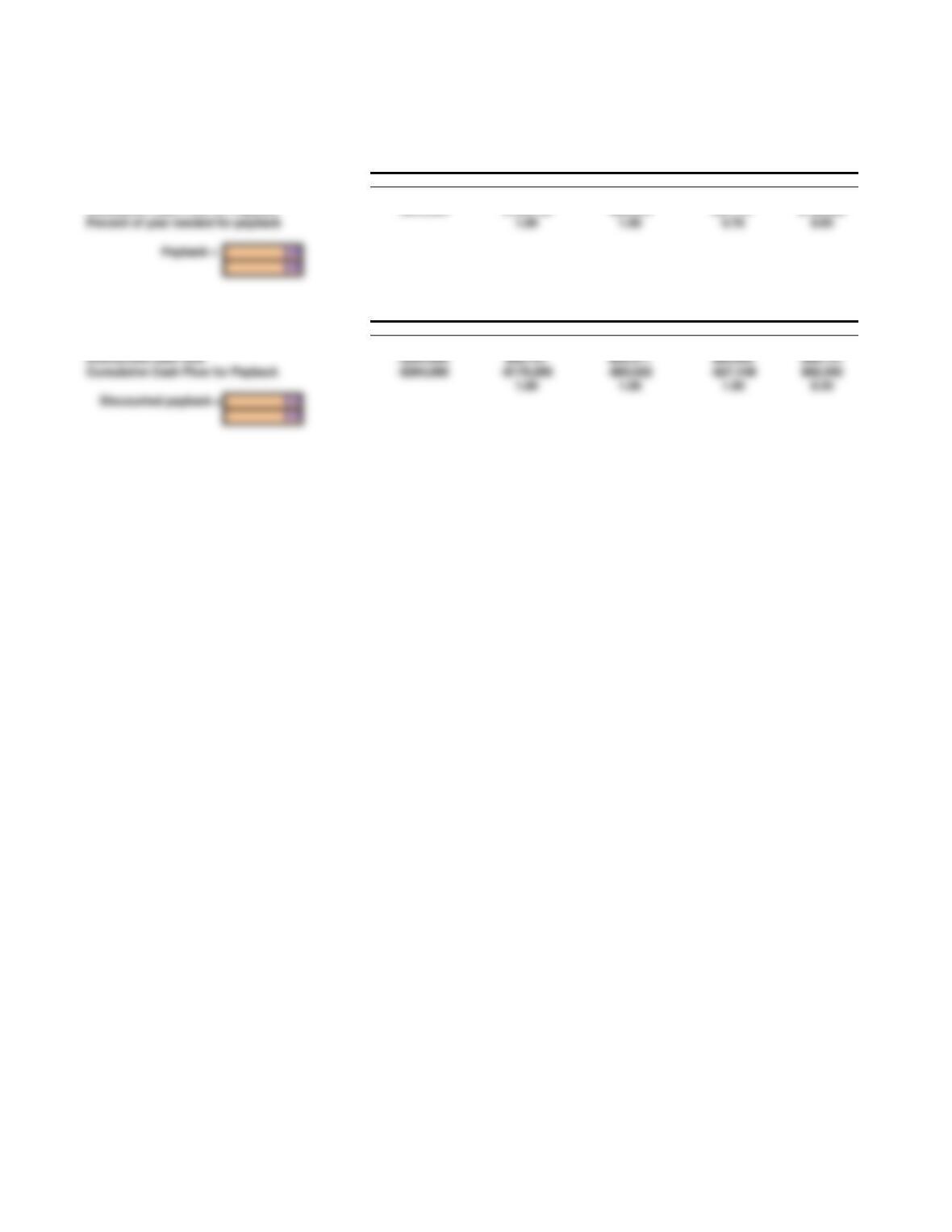
Find Payback
0 1 2 3 4
Cash Flow -$264,000 $94,278 $103,178 $87,691 $131,376
Cumulative Cash Flow for Payback -$264,000 -$169,722 -$66,544 $21,147 $152,522
Percent of year needed for payback 1.00 1.00 0.76 0.00
Find Discounted Payback
0 1 2 3 4
Cash Flow -$264,000 $94,278 $103,178 $87,691 $131,376
Discounted cash flow -$264,000 $85,707 $85,271 $65,883 $89,731
Cumulative Cash Flow for Payback -$264,000 -$178,293 -$93,022 -$27,138 $62,593
Years
Years
% Deviation
% Deviation
% Deviation
from Base cost NPV from Base units NPV from Base Salv. NPV
Base Case $100 $62,593 Base Case 1,000 $62,593 Base Case $25,000 $62,593
-30% $70 $136,927 -30% 700 -$9,363 -30% $17,500 $58,751
-15% $85 $99,760 -15% 850 $26,615 -15% $21,250 $60,672
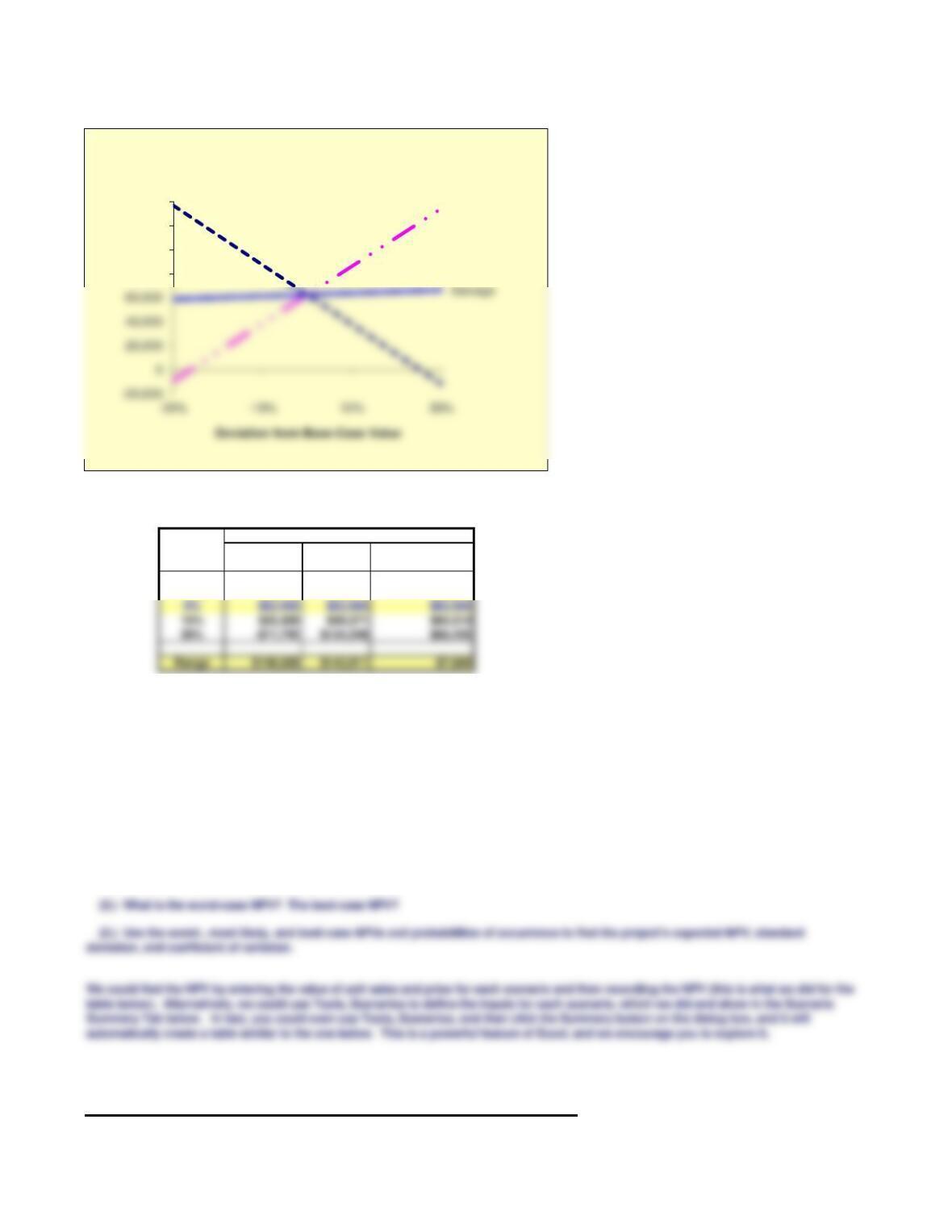
We summarize the data tables and show the sensitivity analysis graph below:
1st YEAR UNIT SALES
SALVAGE
j. (1.) What is sensitivity analysis? Answer: See Chapter 11 Mini Case Show
Incremental Costs
Here we use an Excel “Data Table” to find the NPVs for changes in unit sales, salvage value, and WACC holding other things constant–
changing one variable at a time. This produces the sensitivity analys as shown below.
(2.) Perform a sensitivity analysis on the unit sales, salvage value, and cost of capital for the project. Assume that each of these
variables can vary from its base-case, or expected, value by plus and minus 10%, 20%, and 30%. Include a sensitivity diagram, and
discuss the results.
(2.) How is each of these risk types measured, and how do they relate to one another? Answer: See Chapter 11 Mini Case Show
(3.) How is each type of risk used in the capital budgeting process? Answer: See Chapter 11 Mini Case Show
h. What does the term ”risk” mean in the context of capital budgeting; to what extent can risk be quantified; and when risk is quantified, is
the quantification based primarily on statistical analysis of historical data or on subjective, judgmental estimates?
Answer: See Chapter 11 Mini Case Show
i. (1.) What are the three types of risk that are relevant in capital budgeting? Answer: See Chapter 11 Mini Case Show
Deviation NPV Deviation from Base Case
from
Base Case Cost per unit Units Sold Salvage
-30% $136,927 -$9,363 $58,751
-15% $99,760 $26,615 $60,672
Scenario Analysis
Probability Unit Sales Unit Price NPV
Scenario
deviation, and coefficient of variation.
Squared Deviation
times Probability
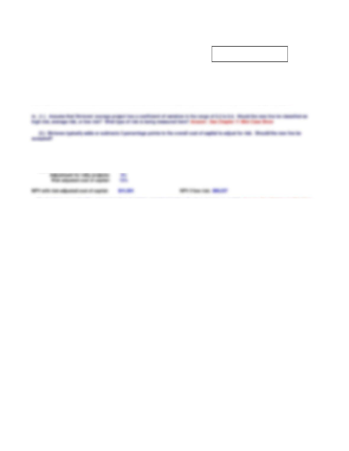
Scenario analysis extends risk analysis in two ways: (1) It allows us to change more than one variable at a time, hence to see the combined
effects of changes in several variables on NPV, and (2) it allows us to bring in the probabilities of changes in the key variables.
(3.) What is the primary weakness of sensitivity analysis? What is its primary usefulness? Answer: See Chapter 11 Mini Case Show
k. Assume that Sidney Johnson is confident of her estimates of all the variables that affect the project’s cash flows except unit sales and
sales price: If product acceptance is poor, unit sales would be only 800 units a year and the unit price would only be $160; a strong
consumer response would produce sales of 1,200 units and a unit price of $240. Sidney believes that there is a 25% chance of poor
acceptance, a 25% chance of excellent acceptance, and a 50% chance of average acceptance (the base case).
(1.) What is scenario analysis?
Cost per unit Units Sold
80,000
100,000
120,000
140,000
NPV ($)
Sensitivity Analysis
25% 1,200 $240 $227,595
50% 1,000 $200 $62,593
25% 800 $160 -$63,399
Quick calculation:
Expected NPV = $72,345 $72,345
Standard Deviation = 103,343 103,343
Coefficient of Variation = Std Dev / Expected NPV = 1.43
Cost of capital for average projects: 10%
The CV of this project is 1.43, which is larger than the CV range of the firm’s average project. Consequently, this project is riskier than the
firm’s average project, so management should add 3% to the WACC to risk adjust.
n. What is a real option? What are some types of real options? Answer: See Chapter 11 Mini Case Show
(2.) Shrieves typically adds or subtracts 3 percentage points to the overall cost of capital to adjust for risk. Should the new line be
m. (1.) Assume that Shrieves‘ average project has a coefficient of variation in the range of 0.2 to 0.4. Would the new line be classified as
(3.) Are there any subjective risk factors that should be considered before the final decision is made? Answer: See Chapter 11 Mini Case
Show
$47,557,148.53
$4,606,631,706.48
Best Case
Base Case
Worst Case
l. Are there problems with scenario analysis? Define simulation analysis, and discuss its principal advantages and disadvantages. Answer:
See Chapter 11 Mini Case Show. Also, see the worksheet this file for an application of simulation analysis to this project analysis.
$6,025,613,876.98
Scenario Summary
Current Values: Base Case Best Case Worst Case
Changing Cells:
$D$35 Base Case Base Case Best Case Worst Case
$D$36 $200,000 $200,000 $200,000 $200,000
$D$37 $10,000 $10,000 $10,000 $10,000
$D$38 $30,000 $30,000 $30,000 $30,000
$D$39 4 4 4 4
$D$40 $25,000 $25,000 $25,000 $25,000
$D$41 25% 25% 25% 25%
$D$42 10% 10% 10% 10%
$D$46 12% 12% 12% 12%
Result Cells:
$H$36 $62,593 $62,593 $227,595 ($63,399)
11/21/2018
Part I: Input Data
Scenario: Base Case
Equipment cost $200,000 Key Outputs: NPV = ($60,457)
Shipping charge $10,000
Installation charge $30,000
Economic Life 4
Salvage Value $25,000
Tax Rate 25% Simulation Inputs
Units Sold 638 Units sold: ######### 200
Sales Price Per Unit $176.74 Sales price/unit: ######### $30
Incremental Cost Per Unit $100
Inflation rate 3%
Annual Depreciation Expense
Depreciable Basis = Equipment + Freight + Installation
Depreciable Basis = $240,000
Year 1 Year 2 Year 3 Year 4
Basis $240,000
Depreciation rate 0.3333 0.4445 0.1481 0.0741
Depreciation expense $79,992 $106,680 ######### $17,784
Remaining book value $160,008 $53,328 ######### $0
Annual Operating Cash Flows
Year 1 Year 2 Year 3 Year 4
Units 638 638 638 638
Unit price $177 $182 $188 $193
Unit cost $100 $103 $106 $109
Sales $112,718 $116,099 $119,582 $123,170
Depreciation $79,992 $106,680 $35,544 $17,784
Operating income before taxes (EBIT) -$31,049 -$56,269 $16,380 $35,697
Taxes (25%) -$7,762 -$14,067 $4,095 $8,924
Net operating profit after taxes (NOPAT) -$23,287 -$42,202 $12,285 $26,773
Net operating profit after taxes (NOPAT) -$23,287 -$42,202 $12,285 $26,773
Operating cash flow $56,705 $64,478 $47,829 $44,557
Annual Cash Flows due to Investments in Net Working Capital
Year 0 Year 1 Year 2 Year 3 Year 4
Sales $112,718 $116,099 $119,582 $123,170
d. Calculate annual net operating profit after sales (NOPAT).
cash flows? See answer to part d.
e. Estimate the required net operating working capital (NOWC) for each year, and the cash flow due to investments in net working
capital.
Monte Carlo simulation is similar to scenario analysis in that different values of key inputs are used Unlike scenario analysis, Monte
Carlo simulation draws a trial set of input values from specified probability distributions and then computes the NPV for this trial. This
process is repeated for hundreds, or even thousands, of trials, with key results (like NPV) saved from each trial. After running the
number of desired trials, the NPVs from the trials can be averaged to estimate the project’s expected NPV; the trial results can also be
used to provide a histogram showing the project’s possible outcomes.
b. Disregard the assumptions in Part a. What is Shrieves’ depreciable basis? What are the annual
11/21/2018
Year 2018 2019 2020 2021 2022 2023 2024 2025 2026 2027
2020 When asset placed in service
2020 2021 2022 2023
Initial basis for depreciation $100,000
Bonus depreciation rate: 100%
Bonus depreciation: $100,000
Remaining MACRS basis: $0
Annual MACRS depreciation rate 33.33% 44.45% 14.81% 7.41%
Annual MACRS depreciation expense $0 $0 $0 $0
Total depreciation expense: $100,000 $0 $0 $0
Remaining undepreciated value (book value)
2023 When asset placed in service
2023 2024 2025 2026
Initial basis for depreciation $100,000
Bonus depreciation rate: 80%
Bonus depreciation: $80,000
Remaining MACRS basis: $20,000
Annual MACRS depreciation rate 33.33% 44.45% 14.81% 7.41%
Annual MACRS depreciation expense $6,666 $8,890 $2,962 $1,482
Total depreciation expense: $86,666 $8,890 $2,962 $1,482
Remaining undepreciated value (book value)
Bonus depreciation allows a company to take additional depreciation in the year that an asset is put in
service. Following are the bonus depreciation rates for assets placee in service in the following years:
Suppose an asset is acquired in 2018 and has a $100,000 basis. It has a 3-year classification.
What is the total depreciation expense each year? What is the total depreciation expense if the
asset is acquired in 2022? In 2023?
Bonus Depreciation in the 2017 Tax Cuts and Job Act (TCJA)