Chapter 11
Cash Flow Estimation and
Risk Analysis
ANSWERS TO END-OF-CHAPTER QUESTIONS
11-1 a. Project cash flow, which is the relevant cash flow for project analysis, represents the
actual flow of cash, which includes investments in capital and working capital, but does
b. Incremental cash flows are those cash flows that arise solely from the asset that is being
evaluated. For example, assume an existing machine generates revenues of $1,000 per
year and expenses of $600 per year. A machine being considered as a replacement would
generate revenues of $1,000 per year and expenses of $400 per year. On an incremental
basis, the new machine would not increase revenues at all, but would decrease expenses
by $200 per year. Thus, the annual incremental cash flow is a before-tax savings of $200.
A sunk cost is one that has already occurred and is not affected by the capital project
decision. Sunk costs are not relevant to capital budgeting decisions. Within the context
of this chapter, an opportunity cost is a cash flow that a firm must forgo to accept a
c. Net operating working capital changes are the increases in current operating assets
resulting from accepting a project less the resulting increases in current operating
liabilities, or accruals and accounts payable. A net operating working capital change
d. Stand-alone risk is the risk a project would have if it was held in isolation. Corporate
(within-firm) risk is the risk that a project contributes to a company after taking into
consideration the cash flows of the company’s other projects; because projects are not
perfectly correlated, corporate risk usually will be less than stand-alone risk. Market
(beta) risk is the risk that a company contributes to a well diversified portfolio.
f. A risk-adjusted discount rate incorporates the risk of the project’s cash flows. The cost
of capital to the firm reflects the average risk of the firm’s existing projects. Thus, new
projects that are riskier than existing projects should have a higher risk-adjusted discount
rate. Conversely, projects with less risk should have a lower risk-adjusted discount rate.
This adjustment process also applies to a firm’s divisions. Risk differences are difficult
to quantify, thus risk adjustments are often subjective in nature. A project’s cost of
capital is its risk-adjusted discount rate for that project.
h. Real options occur when managers can influence the size and risk of a project’s cash
flows by taking different actions during the project’s life. They are referred to as real
options because they deal with real as opposed to financial assets. They are also called
managerial options because they give opportunities to managers to respond to changing
market conditions. Sometimes they are called strategic options because they often deal
with strategic issues. Finally, they are also called embedded options because they are a
part of another project.
11-2 Only cash can be spent or reinvested, and since accounting profits do not represent cash, they
are of less fundamental importance than cash flows for investment analysis. Recall that in
the stock valuation chapters we focused on dividends and free cash flows, which represent
cash flows, rather than on earnings per share, which represent accounting profits.
11-4 Capital budgeting analysis should only include those cash flows which will be affected by
the decision. Sunk costs are unrecoverable and cannot be changed, so they have no bearing
on the capital budgeting decision. Opportunity costs represent the cash flows the firm gives
up by investing in this project rather than its next best alternative, and externalities are the
cash flows (both positive and negative) to other projects that result from the firm taking on
this project. These cash flows occur only because the firm took on the capital budgeting
project; therefore, they must be included in the analysis.
11-6 Scenario analysis analyzes a limited number of outcomes. Although the base case scenario
may be the most likely, or expected outcome, the bad and good scenarios are frequently worst
case and best case scenarios, that is, when everything goes bad together, or everything goes
11-7 The costs associated with financing are reflected in the weighted average cost of capital.
To include interest expense in the capital budgeting analysis would “double count” the cost
of debt financing.
11-8 Daily cash flows would be theoretically best, but they would be costly to estimate and
probably no more accurate than annual estimates because we simply cannot forecast
11-9 In replacement projects, the benefits are generally cost savings, although the new
machinery may also permit additional output. The data for replacement analysis are
generally easier to obtain than for new products, but the analysis itself is somewhat more
complicated because almost all of the cash flows are incremental, found by subtracting the
new cost numbers from the old numbers. Similarly, differences in depreciation and any
other factor that affects cash flows must also be determined.
11-10 Stand-alone risk is the project’s risk if it is held as a lone asset. It disregards the fact that
it is but one asset within the firm’s portfolio of assets and that the firm is but one stock in
a typical investor’s portfolio of stocks. Stand-alone risk is measured by the variability of
11-11 It is often difficult to quantify market risk. On the other hand, we can usually get a good
idea of a project’s stand–alone risk, and that risk is normally correlated with market risk:
The higher the stand-alone risk, the higher the market risk is likely to be. Therefore, firms
tend to focus on stand-alone risk, then deal with corporate and market risk by making
subjective, judgmental modifications to the calculated stand-alone risk.
SOLUTIONS TO END-OF-CHAPTER PROBLEMS
11-1 a. Equipment $ 17,000,000
NWC Investment 5,000,000
Initial investment outlay $22,000,000
11-2 Operating Cash Flows: t = 1
Sales revenues $18,000,000
Operating costs 9,000,000
Depreciation 4,000,000
Operating income before taxes $ 5,000,000
Taxes (25%) 1,250,000
Operating income after taxes $ 3,750,000
Add back depreciation 4,000,000
Operating cash flow $ 7,750,000
11-3 Equipment’s original cost $12,000,000
Depreciation (80%) 9,000,000
11-4 Cash outflow = $110,000.
Increase in annual after-tax cash flows: CF = $19,000.
Place the cash flows on a time line:
0 1 2 10
| | | • • • |
–110,000 19,000 19,000 19,000
11-5 a. The MACRS rates are 33.33%, 44.45%, 14.81%, and 7.41%. The first MACRS
depreciation expense is 33.33%($1,700,000) = $566,610. The others are calculated
similarly. The applicable depreciation values are as follows for the two scenarios:
Scenario 1 Scenario 2
Year (Straight Line) (MACRS)
1 $425,000 $566,610
b. To find the difference in net present values under these two methods, we must determine
the difference in incremental cash flows each method provides. The depreciation
expenses cannot simply be subtracted from each other, as there are tax ramifications due
to depreciation expense. The full depreciation expense is subtracted from Revenues to
10
Depreciation Expense Depreciation Expense
Year Difference (2 – 1) Diff. 0.25 (MACRS)
1 $141,610 $35,402.5
2 330,650 82,662.5
Now to find the difference in NPV to be generated under these scenarios, just enter the
cash flows that represent the benefit from depreciation expense and solve for net present
value based upon a cost of capital of 10%.
CF0 = 0; CF1 = 35402.5; CF2 = 82662.5; CF3 = -43307.5; CF4 = -74757.5; and I/YR =
10. Solve for NPV = $16,902.26
So, all else equal the use of the accelerated depreciation method will result in a higher
NPV (by $16,902.26) than would the use of a straight-line depreciation method.
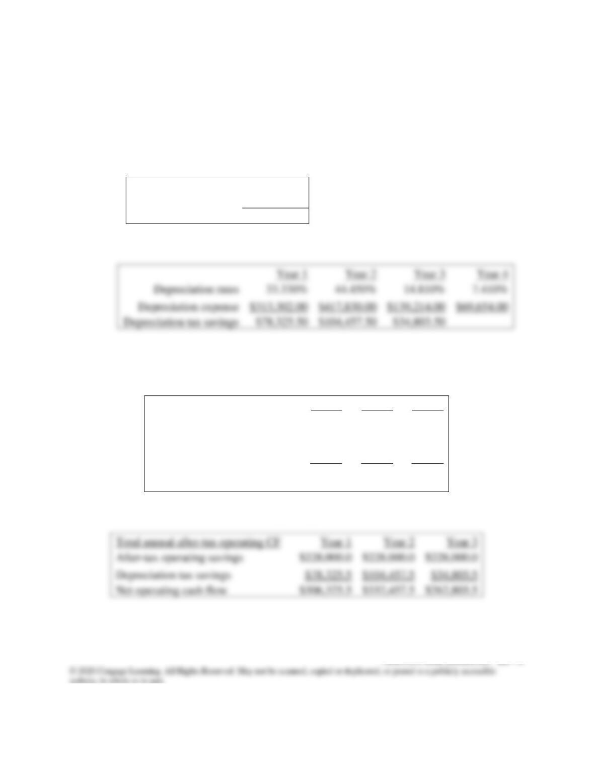
11-6 a. The net initial cash flow is:
Machine price
−$920,000
Installation cost
−$20,000
NWC required
−$15,500
b. The operating cash flows are:
First, calculate deprecation basis, annual depreciation expenses, and the annual tax
savings due to depreciation. The tax rate is 25%.
Basis:
Machine cost
920,000
Installation expense
20,000
Depreciation basis
940,000
Depreciation tax savings:
$313,302.00
$417,830.00
$139,214.00
$69,654.00
$104,457.50
Second, calculate the after-tax operating savings.
Year 1
Year 2
Year 3
Before-tax operating savings
304,000
304,000
304,000
Tax on operating savings
76,000
76,000
76,000
After-tax operating savings
228,000
228,000
228,000
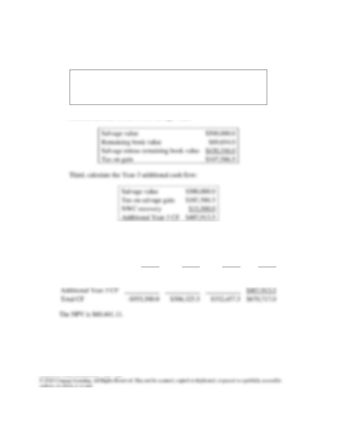
Third, calculate the total annual operating cash flows.
Total annual after-tax operating CF
After-tax operating savings
$228,000.0
$228,000.0
$228,000.0
Depreciation tax savings
$104,457.5
Net operating cash flow
$306,325.5
$332,457.5
$262,803.5
c. The additional Year-3 cash flows are:
First, find the remaining book value:
Salvage value calculation
Additional Year-3 CF
Depreciation basis
$940,000.0
Total depreciation expense in Years 1 through 3
$870,346.0
Remaining book value
$69,654.0
Salvage value
$500,000.0
Remaining book value
Salvage minus remaining book value
$430,346.0
Tax on gain
$107,586.5
Salvage value
$500,000.0
Tax on salvage gain
$107,586.5
NWC recovery
Additional Year-3 CF
$407,913.5
d. The cost of capital is 12%.
The total annual cash flows are:
Year 0
Year 1
Year 2
Year 3
Year 0 CF
-$955,500.0
Net operating CF
$306,325.5
$332,457.5
$262,803.5
Additional Year-3 CF
$407,913.5
Total CF
-$955,500.0
$306,325.5
$332,457.5
$670,717.0
11-7 The net cost is $89,000:
Basic price
$70,000.00
Modifications
$15,000.00
NWC increase
$4,000.00
Time 0 CF
$89,000.00
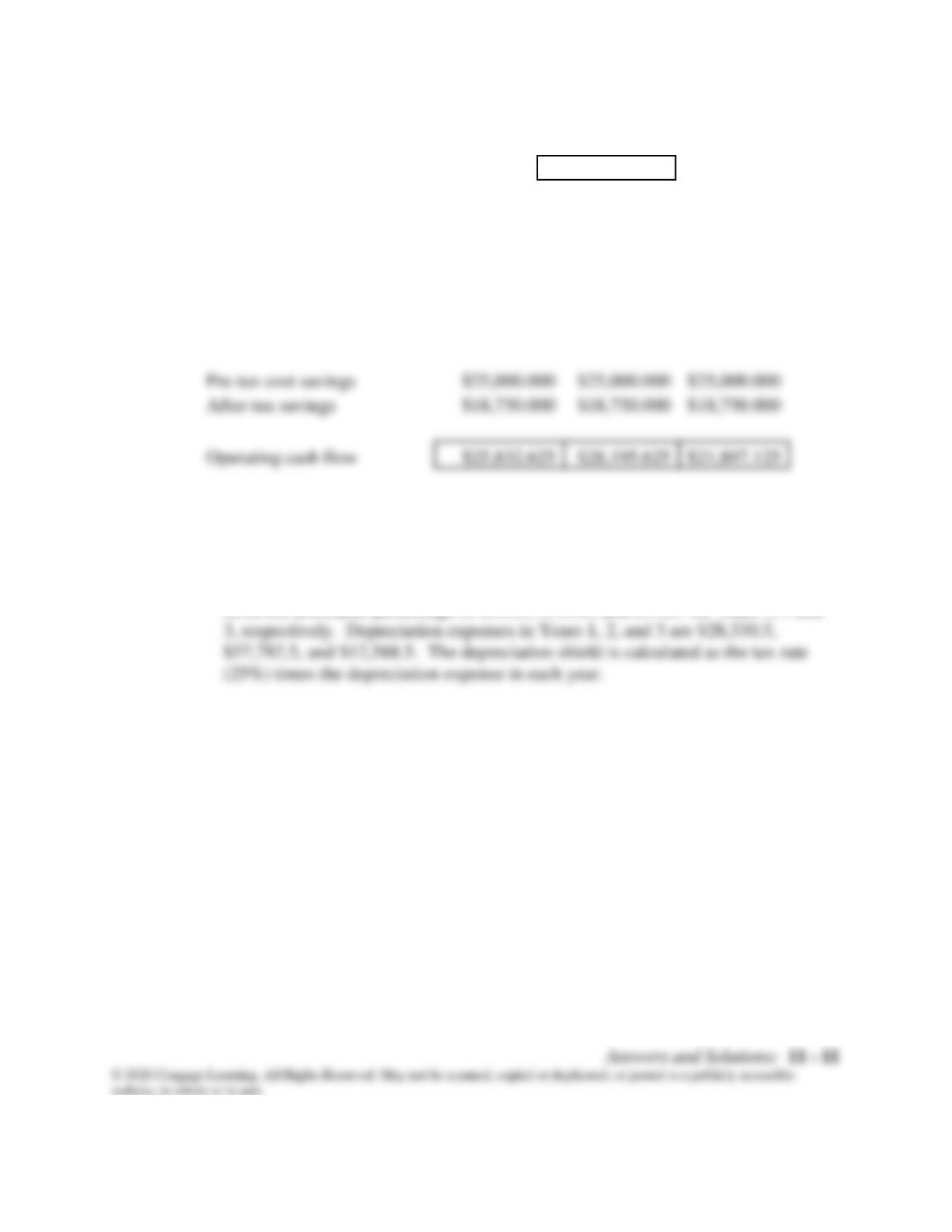
b. The operating cash flows follow:
Depreciation basis
$85,000.000
1
2
3
Depreciation expenses
$28,330.500
$37,782.500
$12,588.500
Depreciation tax shield
$7,082.625
$9,445.625
$3,147.125
After-tax savings
$18,750.000
$18,750.000
$18,750.000
Operating cash flow
$28,195.625
$21,897.125
Notes:
1. The after-tax cost savings is $25,000(1 – T) = $25,000(0.75) = $18,750.
2. The depreciation expense in each year is the depreciable basis, $85,000, times the
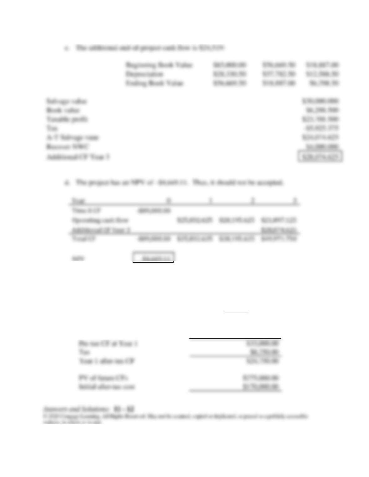
Beginning Book Value
Depreciation
Ending Book Value
Salvage value
Book value
Taxable profit
Tax
A-T Salvage vaue
Recover NWC
Additional CF Year 3
$28,074.625
11-8 a.
Year1 sales = 1,000($138)$138,000
Year-1 costs = 1,000($105)105,000
Sales revenues at Year 1
$138,000.00
Costs at Year 1
$105,000.00
Pre-tax CF at Year 1
Tax
Year 1 after-tax CF
PV of future CFs
$275,000.00
Initial after-tax cost
$170,000.00
NPV
$105,000.00
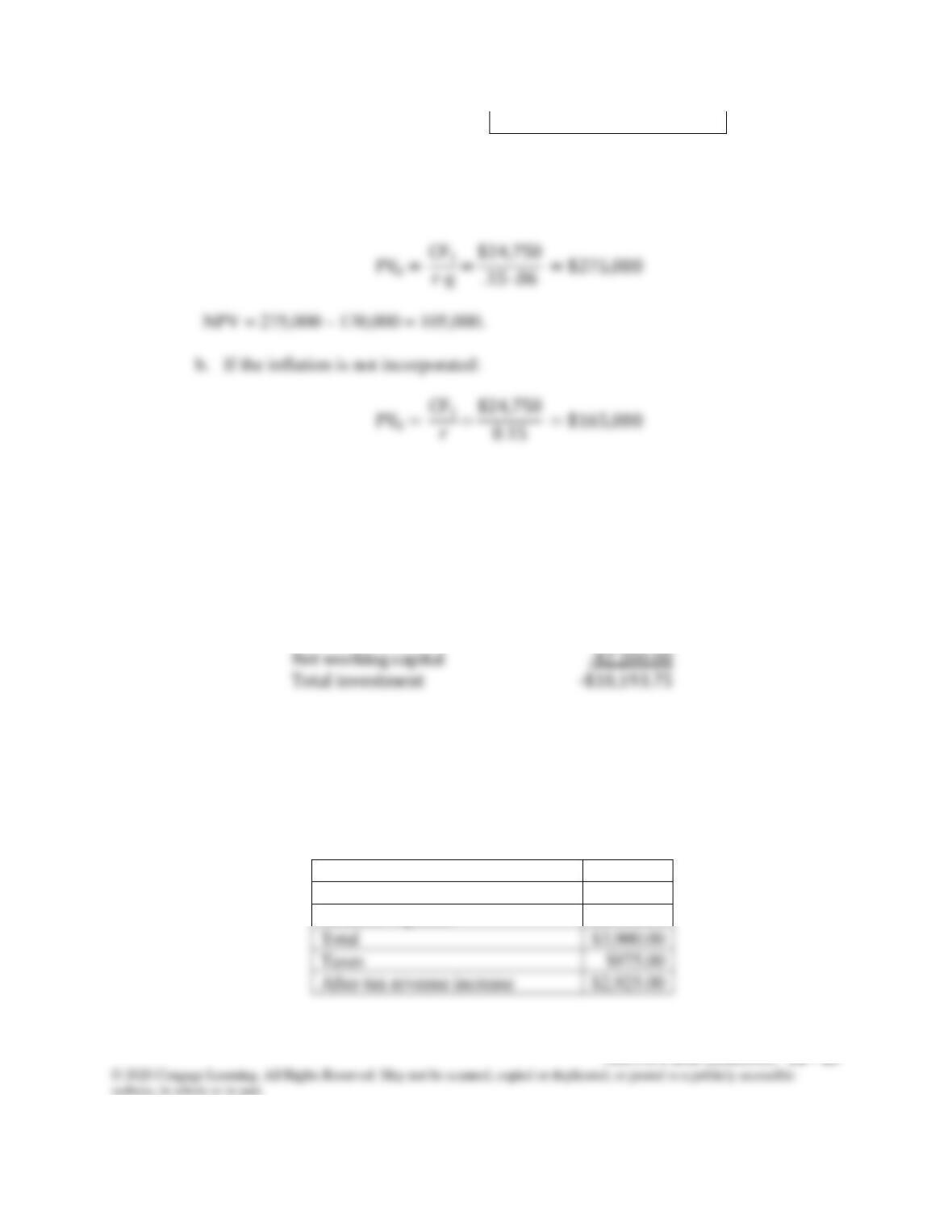
Using the Year-1 price and theconstant growth formula , the present value of all of
the future cash flows is:
NPV = 165,000 – 170,000 = −$5,000.
11-9 First determine the net cash flow at t = 0:
CF0 Calculation
Purchase Price
-$12,000.00
Sale of old machine
$4,150.00
Tax on sale
-$143.75
Net working capital
Total investment
a The market value is $4,150 – $3,575 = $575 above the book value. Thus, there is a $575
recapture of depreciation, and Gilbert would have to pay 0.25($575) = $143.75 in taxes.
b The change in net working capital is a $2,900 increase in current assets minus a $700
increase in current liabilities, which totals to $2,200.
Annual after-tax revenue increases
Sales increase
$2,000.00
Reduced expenses
$1,900.00
Total
$3,900.00
Taxes
After-tax revenue increase
$2,925.00
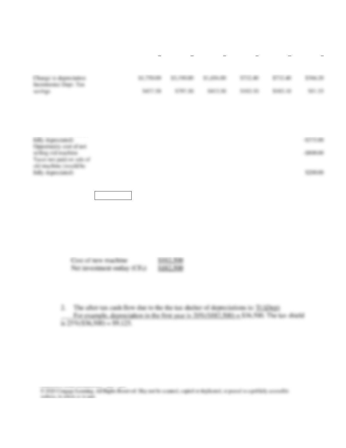
Year
1
2
3
4
5
6
New depreciation
$2,400.00
$3,840.00
$2,304.00
$1,382.40
$1,382.40
$691.20
Old depreciation
$650.00
$650.00
$650.00
$650.00
$650.00
$325.00
Change in depreciation
$1,750.00
$3,190.00
$1,654.00
$732.40
$732.40
$366.20
Incremental Depr. Tax
savings
$437.50
$797.50
$413.50
$183.10
$183.10
Recover NWC
$2,200.00
Sell replacement
machine
$1,500.00
Tax on sale of
replacement machine (is
selling old machine
$200.00
Total CFs
-$10,193.75
$3,362.50
$3,722.50
$3,338.50
$3,108.10
$3,108.10
$5,741.55
NPV
$3,544.60
11–10 1. Net investment at t = 0:
2. The after-tax earnings are
($74,000 − $27,000) (1 – T) = $47,000(0.75) = $35,250
Year
Initial
investment
Depreciation
Increase
in ebitda
after tax
Increase in
depreciation
tax shield
Total CF
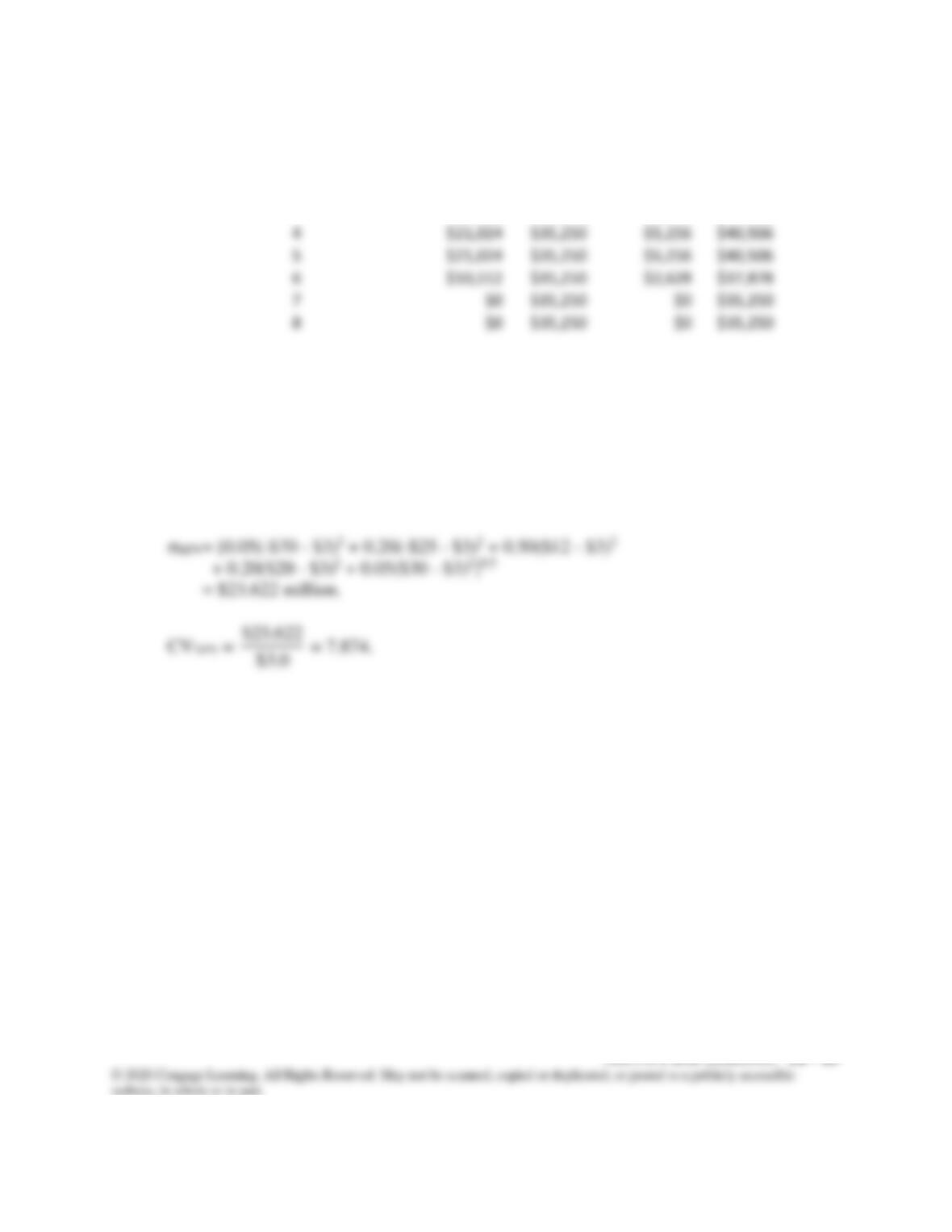
0
$182,500
–
$182,500
1
$36,500
$35,250
$9,125
$44,375
2
$58,400
$35,250
$14,600
$49,850
3
4
$21,024
$35,250
$5,256
$40,506
5
$21,024
$35,250
$5,256
$40,506
6
$10,512
$35,250
$2,628
$37,878
7
$35,250
$35,250
8
$35,250
$35,250
$35,040
$35,250
$8,760
$44,010
The NPV of the total CFs using a 12% cost of capital is $26,285.
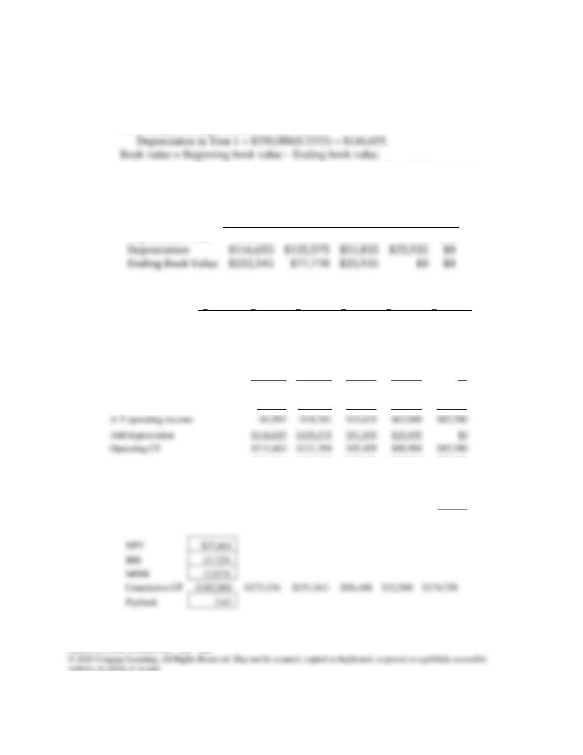
11-11 E(NPV) = 0.05(-$70) + 0.20(-$25) + 0.50($12) + 0.20($20) + 0.05($30)
= -$3.5 + -$5.0 + $6.0 + $4.0 + $1.5
= $3.0 million.
11-12 a. First, set up a depreciation schedule.
Depreciation basis = $350,000.
Depreciation = Basis(Depreciation rate)
For example, the depreciation in Year 1 is:
At Year 1, the ending value is equal to the basis minus the depreciation expense:
$350,000 – $116,655 = $233,345.
Then beginning basis for a year is equal to the ending basis for the previous year.
1
2
3
4
5
Depreciation rate
33.33%
44.45%
14.81%
7.41%
0%
Depreciation
$116,655
$155,575
$51,835
$25,935
Ending Book Value
$233,345
$25,935
0
1
2
3
4
5
Machine cost
-$350,000
Net working capital
-$35,000
Cost savings
$110,000
$110,000
$110,000
$110,000
$110,000
Depreciation
$116,655
$155,575
$51,835
$25,935
$0
Op. Inc. before taxes
-$6,655
-$45,575
$58,165
$84,065
$110,000
Taxes
-$1,664
-$11,394
$14,541
$21,016
$27,500
A-T operating income
-$4,991
-$34,181
$43,624
$63,049
$82,500
Add depreciation
$116,655
$155,575
$51,835
$25,935
$0
Operating CF
$111,664
$121,394
$95,459
$88,984
$82,500
$111,664
$121,394
$95,459
$88,984
$82,500
Return of NWC
$35,000
Sale of machine
$33,000
Tax on sale
-$8,250
Total CF
-$385,000
$111,664
$121,394
$95,459
$88,984
$142,250
NPV
IRR
MIRR
Cumulative CF
-$385,000
-$273,336
-$151,943
-$56,484
$32,500
$174,750
Payback
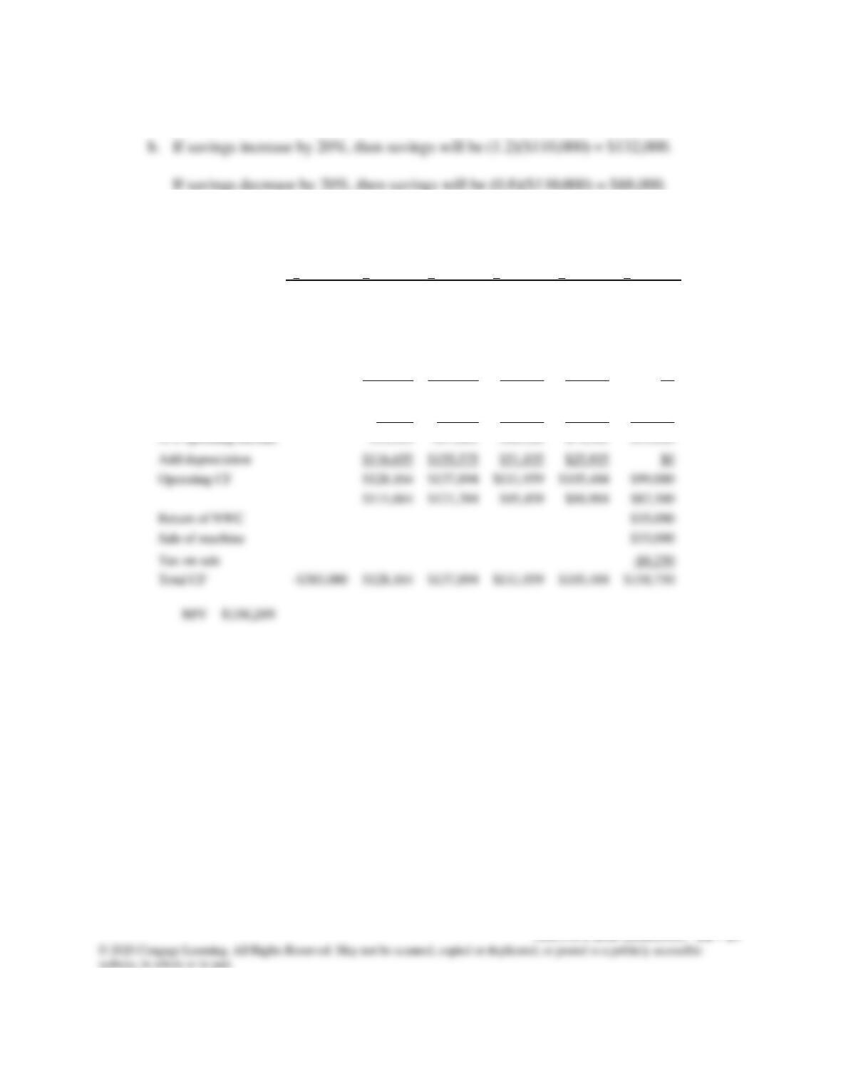
(1) Savings increase by 20%:
0
1
2
3
4
5
Machine cost
-$350,000
Net working capital
-$35,000
Cost savings
$132,000
$132,000
$132,000
$132,000
$132,000
Depreciation
$116,655
$155,575
$51,835
$25,935
$0
Op. Inc. before taxes
$15,345
-$23,575
$80,165
$106,065
$132,000
Taxes
$3,836
-$5,894
$20,041
$26,516
$33,000
A-T operating income
$11,509
-$17,681
$60,124
$79,549
$99,000
Add depreciation
$116,655
$155,575
$51,835
$25,935
$0
Operating CF
$128,164
$137,894
$111,959
$105,484
$99,000
$111,664
$121,394
$95,459
$88,984
$82,500
Return of NWC
$35,000
Sale of machine
$33,000
Tax on sale
-$8,250
Total CF
-$385,000
$128,164
$137,894
$111,959
$105,484
$158,750
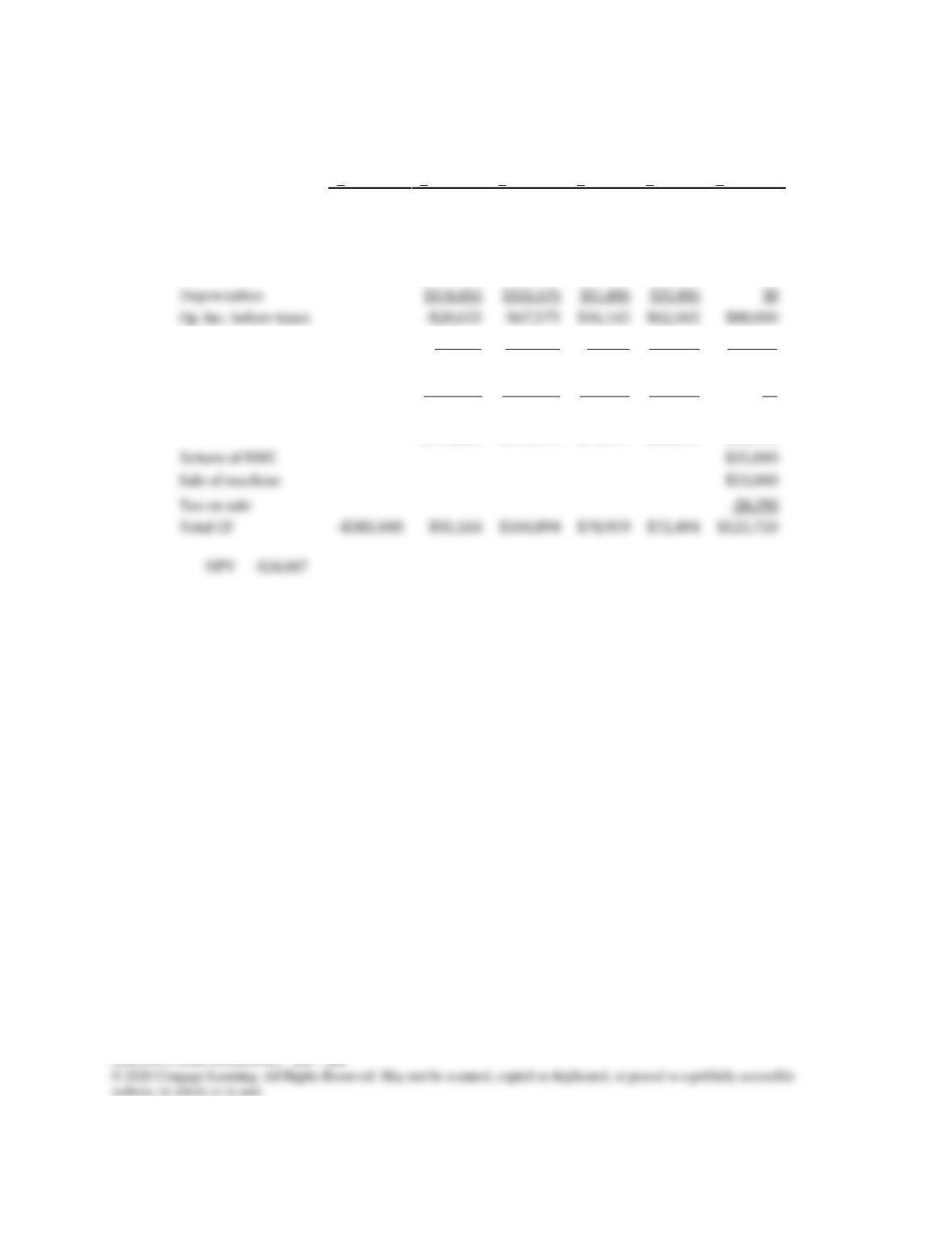
(2) Savings decrease by 20%:
0
1
2
3
4
5
Machine cost
-$350,000
Net working capital
-$35,000
Cost savings
$88,000
$88,000
$88,000
$88,000
$88,000
Depreciation
$116,655
$155,575
$51,835
$25,935
$0
Op. Inc. before taxes
-$28,655
-$67,575
$36,165
$62,065
$88,000
Taxes
-$7,164
-$16,894
$9,041
$15,516
$22,000
A-T operating income
-$21,491
-$50,681
$27,124
$46,549
$66,000
Add depreciation
$116,655
$155,575
$51,835
$25,935
$0
Operating CF
$95,164
$104,894
$78,959
$72,484
$66,000
$111,664
$121,394
$95,459
$88,984
$82,500
Return of NWC
$35,000
Sale of machine
$33,000
Tax on sale
-$8,250
Total CF
-$385,000
$95,164
$104,894
$78,959
$72,484
$125,750
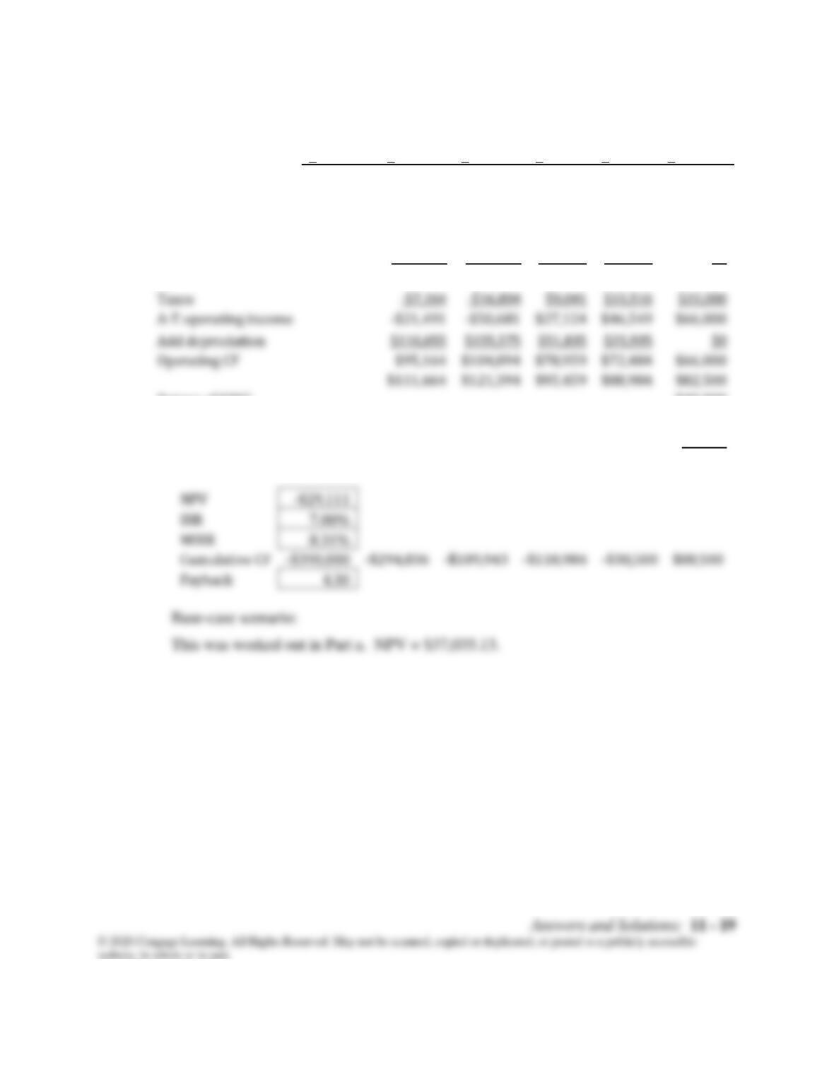
c. Worst-case scenario:
0
1
2
3
4
5
Machine cost
-$350,000
Net working capital
-$40,000
Cost savings
$88,000
$88,000
$88,000
$88,000
$88,000
Depreciation
$116,655
$155,575
$51,835
$25,935
$0
Op. Inc. before taxes
-$28,655
-$67,575
$36,165
$62,065
$88,000
Taxes
-$7,164
$15,516
A-T operating income
-$21,491
-$50,681
$27,124
$46,549
$66,000
Add depreciation
$116,655
$155,575
$51,835
$25,935
$0
Operating CF
$95,164
$104,894
$78,959
$72,484
$66,000
$111,664
$121,394
$95,459
$88,984
$82,500
Return of NWC
$40,000
Sale of machine
$28,000
Tax on sale
-$7,000
Total CF
-$390,000
$95,164
$104,894
$78,959
$72,484
$127,000
NPV
-$29,111
Payback
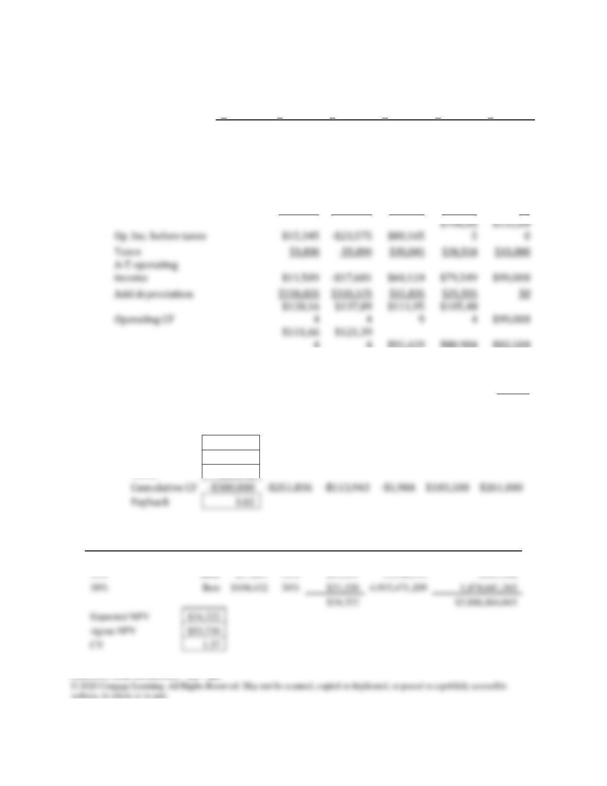
Best-case scenario:
0
1
2
3
4
5
Machine cost
–
$350,000
Net working capital
-$30,000
Cost savings
$132,00
0
$132,00
0
$132,00
0
$132,00
0
$132,00
0
Depreciation
$116,655
$155,575
$51,835
$25,935
$0
Op. Inc. before taxes
$15,345
$80,165
$106,06
5
$132,00
0
Taxes
-$5,894
$20,041
$26,516
$33,000
$11,509
$60,124
$79,549
$99,000
Add depreciation
$51,835
$25,935
$0
Operating CF
$128,16
$137,89
$111,95
$105,48
$99,000
$111,66
$121,39
4
4
$95,459
$88,984
$82,500
Return of NWC
$30,000
Sale of machine
$38,000
Tax on sale
-$9,500
Total CF
–
$380,000
$128,16
4
$137,89
4
$111,95
9
$105,48
4
$157,50
0
NPV
$104,432
IRR
20.18%
MIRR
15.47%
Cumulative CF
-$380,000
-$251,836
-$113,943
-$1,984
$103,500
$261,000
Scenario probabilities
NPV
Prob.
Prob x NPV
Dev. Squared
Prob(Dev. Squared)
35%
Worst
-$29,111
35%
-$10,189
4,023,775,752
1,408,321,513
35%
35%
30%
30%
4,915,471,209
1,474,641,363
$2,886,864,043
Expected NPV
$34,322
sigma NPV
$53,730