CFIN6 – CHAPTER 10
INTEGRATIVE PROBLEMS SOLUTIONS
Integrative Problem 10-1
a. You might want to begin discussion differentiating between cash flow versus accounting income.
b(1). This answer requires no explanation. Students might note, though, that inflation is not reflected at this
point. It will be later. The top part of the income statement is:
Unilate’s Silk/Wool Blend Fabric Project ($ thousands)
End of Year: 1 2 3 4
Unit sales (thousands) 100 100 100 100
Price/unit $2.00 $2.00 $2.00 $2.00
Total revenues $200.0 $200.0 $200.0 $200.0
Costs excluding depreciation (20.0) (120.0) (120.0) (120.0)
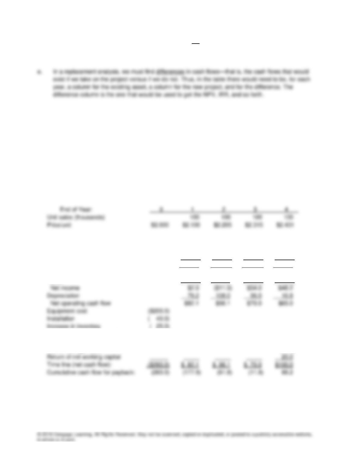
b(3). This is straightforward. The only even slightly complicated thing is adding back depreciation to get net
CF.
Unilate’s Silk/Wool Blend Fabric Project ($ thousands)
End of Year: 0 1 2 3 4
Unit sales (thousands) 100 100 100 100
Price/unit $2.00 $2.00 $2.00 $2.00 $2.00
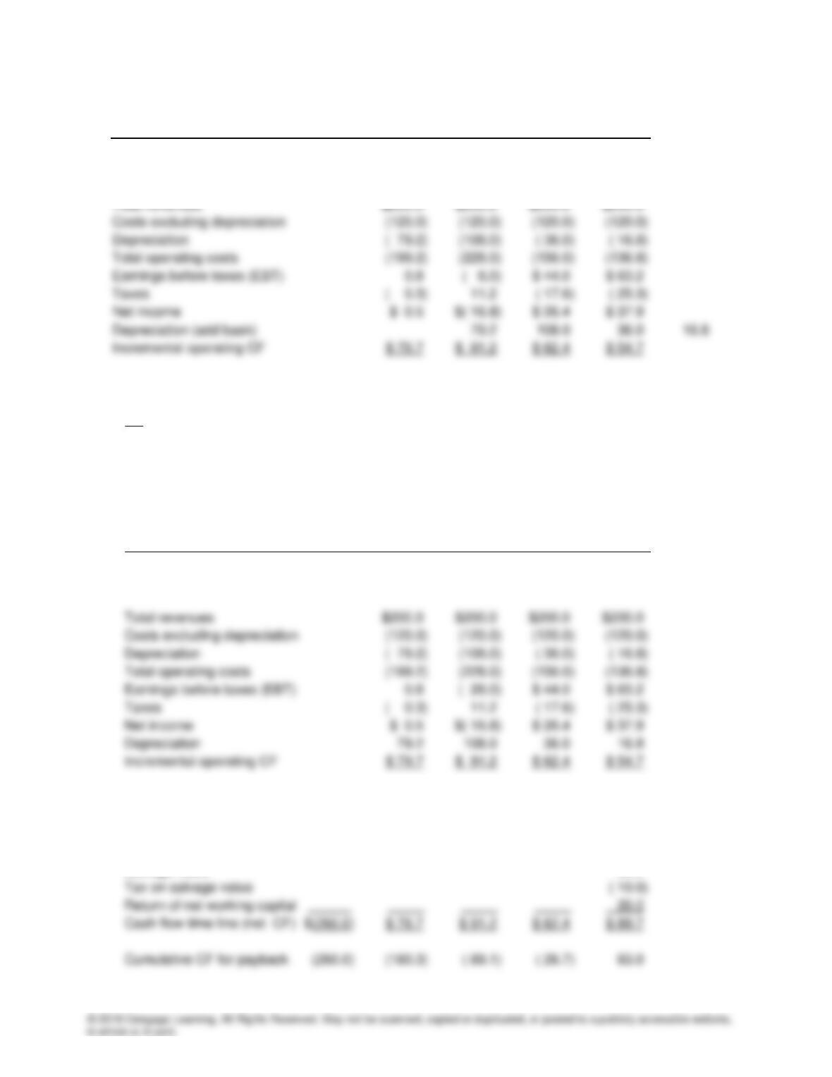
b(4). These are all straightforward. Note that accounts payable is an offset to the inventory buildup, so the
net working capital requirement is $20,000, which is recovered at the end of Year 4. Also, the salvage
value is fully taxable, because the asset has been depreciated to a zero book value. If book value were
something other than zero, the tax effect could be positive (if the asset were sold for less than book
value) or negative.
Unilate’s Silk/Wool Blend Fabric Project ($ thousands)
End of Year: 0 1 2 3 4
Unit sales (thousands) 100 100 100 100
Price/unit $2.00 $2.00 $2.00 $2.00 $2.00
Equipment cost (200.0)
Installation ( 40.0)
Increase in inventory ( 25.0)
Increase in accounts payable 5.0
c(2). This expenditure is a sunk cost, so it would not affect the decision and should not be included in the
analysis.
c(3). The rental payment represents an opportunity cost, and as such its after-tax amount, $25,000(1 – T) =
$25,000(0.6) = $15,000, should be subtracted from the operating cash flows the company would have
otherwise.
d. We refer to the completed cash flow time line and explain how each of the indicators is calculated. We
base our explanation on financial calculators, but it would be equally easy to explain using a regular
calculator and equations.
NPV = -$4.0. NPV is negative; do not accept.
0. =
)
IRR + (1
$89.7
+
)
IRR + (1
$62.4
+
)
IRR + (1
$91.2
+
)
IRR + (1
$79.7
+ $260– :IRR 4321
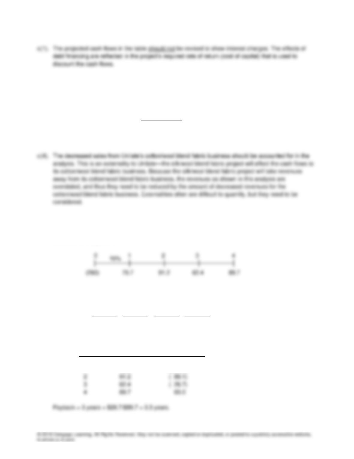
IRR = 9.3%. IRR is less than cost of capital; do not accept.
Payback: Year Cash flow Cumulative Cash Flow
0 $(260.0) $(260.0)
1 79.7 (180.3)
Based on the analysis to this point, the project should not be undertaken. However, this conclusion
might not be correct, as we will see shortly.
f. It is apparent from the data in the previous table that inflation has not been reflected in the calculations.
In particular, the sales price is held constant rather than rising with inflation. Therefore, revenues and
costs (except depreciation) should both be increased by 3% per year. Because revenues are larger
than operating costs, inflation will cause cash flows to increase. This will lead to a higher NPV and
IRR, and to a shorter payback. The following table reflects the changes, and it shows the new cash
flows and the new indicators. When inflation is properly accounted for, the project is seen to be
profitable.
Unilate’s Fabric Project ($ thousands)
Inflation = 3%
Total revenues $210.0 $220.5 $231.5 $243.1
Costs excluding depreciation ( 126.0) ( 132.3) ( 138.9) ( 145.9)
Depreciation ( 79.2) ( 108.0) ( 36.0) ( 16.8)
Total costs ($205.2) ($240.3) ($174.9) ($162.7)
EBT $4.8 ($19.8) $56.6 $80.4
Taxes ( 1.9) 7.9 ( 22.6) ( 32.2)
Increase in accounts payable 5.0
Salvage value 25.0
Tax on salvage value (10.0)
NPV = $15.0
IRR = 12.6%
Payback = 3.1 years

Integrative Problem 10-2
a(1). Here are the three types of project risk:
1. Stand-alone risk is the project’s total risk if it were operated independently. Stand-alone risk
ignores both the firm’s diversification among projects and investors’ diversification among firms.
Stand-alone risk is measured either by the project’s standard deviation (σNPV) or its coefficient of
variation of NPV (cvNPV).
2. Within-firm (corporate) risk is the total riskiness of the project giving consideration to the firm’s
a(2). Because management’s primary goal is shareholder wealth maximization, the most relevant risk for
capital projects is market risk. However, creditors, customers, suppliers, and employees are all
affected by a firm’s total risk. Because these parties influence the firm’s profitability, a project’s
within-firm risk should not be completely ignored.
a(3). By far the easiest type of risk to measure is a project’s stand–alone risk. Thus, firms often focus
a(4). Because most projects that a firm undertakes are in its core business, a project’s stand-alone risk is
likely to be highly correlated with its corporate risk, which in turn is likely to be highly correlated with its
market risk.
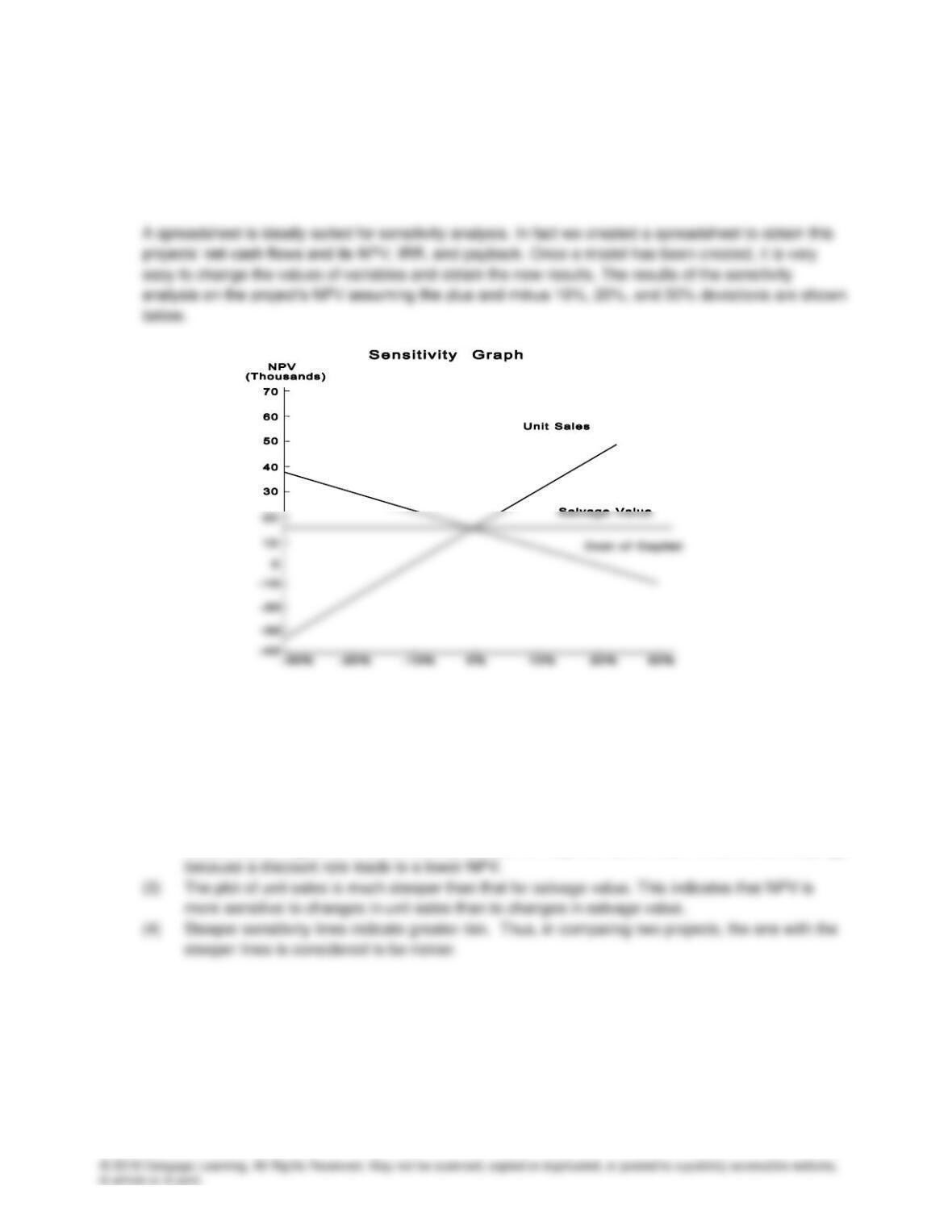
b(1). Sensitivity analysis measures the effect of changes in a particular variable, say revenues, on a
project’s NPV. To perform a sensitivity analysis, all variables are fixed at their expected values except
b(2). The base case value for unit sales was 100; therefore, if you were to assume that this value deviated
by plus and minus 10%, 20%, and 30%, the unit sales values to be used in the sensitivity analysis
would be 70, 80, 90, 110, 120, and 130 units. You would then go back to the table at the beginning of
the problem, insert the appropriate sales unit number, say 70 units, and rework the table for the
variables.) Then, you would go back and repeat the same steps for 80 units—this would be done for
each of the sales unit values. Then, you would repeat the same procedure for the sensitivity analysis
on salvage value and on required rate of return. (Note that for the required rate of return analysis, the
net cash flows would remain the same, but the required rate of return used in the NPV calculations
would be different.)
We generated the data used in the figure that follows with a spreadsheet model.
(1) The sensitivity lines intersect at 0% change and the base case NPV, at approximately $15,000.
Because all other variables are set at their base case, or expected, values, the zero change
situation is the base case.
(2) The plots for unit sales and salvage value are upward sloping, indicating that higher variable
values lead to higher NPVs. Conversely, the plot for required rate of return is downward sloping,
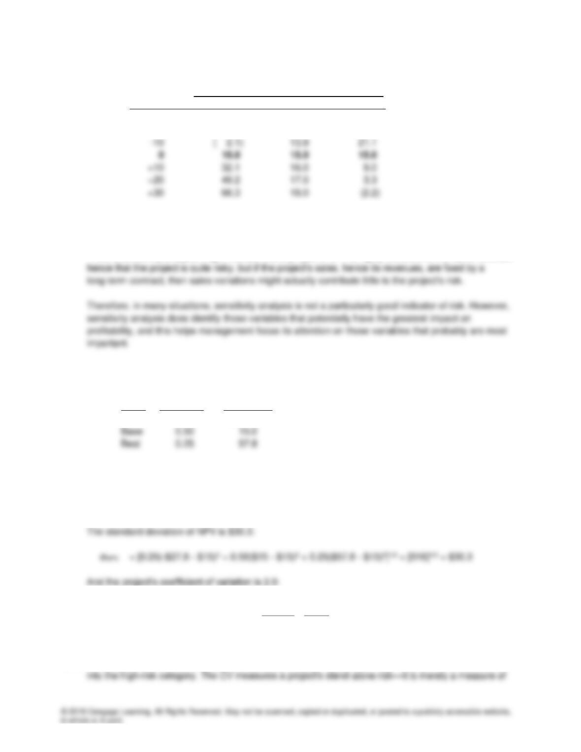
The sensitivity data are given here in tabular form ($ thousands):
Change from Resulting NPV After the Indicated Change in:
Base Level Unit Sales Salvage Value r
-30% ($36.4) $11.9 $34.1
–20 ( 19.3) 12.9 27.5
b(3). The two primary disadvantages of sensitivity analysis are that it does not (1) reflect the effects of
diversification and (2) incorporate any information about the possible magnitudes of the forecast errors.
Thus, a sensitivity analysis might indicate that a project’s NPV is highly sensitive to the sales forecast,
c(1). We used a spreadsheet model to develop the scenarios ($ thousands), which are summarized below:
Case Probability NPV (000s)
Worst 0.25 ($27.8)
c(2). The expected NPV is $14,968 (rounded to the nearest thousand below).
E(NPV) = 0.25(-$27.8) + 0.50($15.0) + 0.25($57.8) = $15.
2.0. =
$15
$30.3
=
E(NPV)
=
CV NPV
NPV
d(1). The project has a CV of 2.0, which is much higher than the average range of 1.25 to 1.75, so it falls
d(2). It is reasonable to assume that if the economy is strong and people are buying a lot of fabric, then
sales would be strong in all of the company’s lines, so there would be positive correlation between this
d(3). If the project’s cash flows are likely to be highly correlated with the firm’s aggregate cash flows, which
generally is a reasonable assumption, then the project would have high corporate risk. However, if the
e(1). In all likelihood, this project would have a positive correlation with returns on other assets in the
economy, and specifically with the stock market. Unilate Textiles produces cloth items, and such firms
e(2). This correlation would not directly affect the project’s corporate risk, but it does, when combined with
the project’s high stand-alone risk, suggest that the project’s market risk as measured by its market
beta is relatively high.
f(1). Because the project is judged to have above-average risk, its differential risk-adjusted, or project,
f(2). A numerical analysis such as this one might not capture all of the risk factors inherent in the project. If
the project has a potential for bringing on harmful lawsuits, then it might be riskier than first assessed.
Also, if the project’s assets can be redeployed within the firm or can be easily sold, then the project
might be less risky than the analysis indicates.
g. Scenario analysis examines several possible scenarios, usually the worst case, the most likely case,
and the best case. Thus, it usually considers only three possible outcomes. Obviously the world is
Although simulation analysis is technically refined, its usefulness is limited because managers often
are unable to accurately specify the variables’ probability distributions. Further, the correlations among
the uncertain variables must be specified, along with the correlations over time. If managers are unable
to do this with much confidence, then the results of simulation analyses are of limited value.
Recognize also that neither sensitivity, scenario, nor simulation analysis provides a decision rule—they
might indicate that a project is relatively risky, but they do not indicate whether the project’s expected
return is sufficient to compensate for its risk.
h(2). Because beta is the measure of market risk, the project’s market risk is 1.2, which indicates that it is
somewhat riskier than the average stock. If Unilate’s beta is less than 1.2, then the new project has
more market risk than the firm’s other assets.
h(3). The project has a CV of 2.0 versus one of about 1.5 for an average project, suggesting that this project
is riskier than the firm’s average project.
h(4). Two methods for estimating a project’s market beta are (1) the pure play method, and (2) the
accounting beta method. In the pure play method, one or more companies that are publicly traded and
are engaged exclusively in the line of business as the project being evaluated are identified. An
average of the betas of these companies is then used as a proxy for the project’s beta. In the

h(5). The advantages of focusing on a project’s market risk are (1) that it is the most relevant risk to
stockholders, hence to determining the effect of the project on the value of the stock, and (2) it results