CHAPTER 3 SOLUTIONS
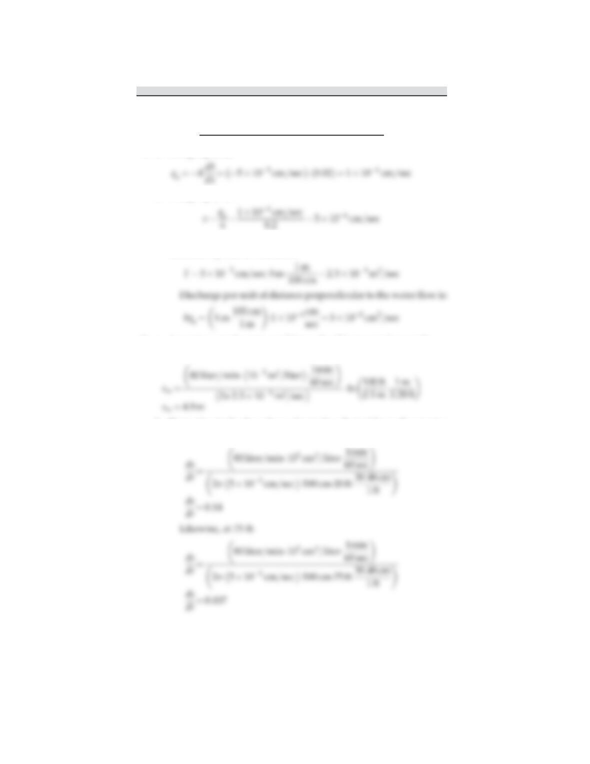
1. a. Using Eq. (3.2):
b. Using Eq. (3.5):
c. Transmissivity is the product of an aquifer’s hydraulic
conductivity and its thickness:
2. a. Assuming steady-state conditions, the Thiem equation can be
applied to estimate the drawdown in the well. Using Eq. (3.8b):
b. First estimate the drawdown due to the effect of the well pumping
by using Eq. (3.7b). At 20 ft:
e67CHAPTER 3 SOLUTIONS
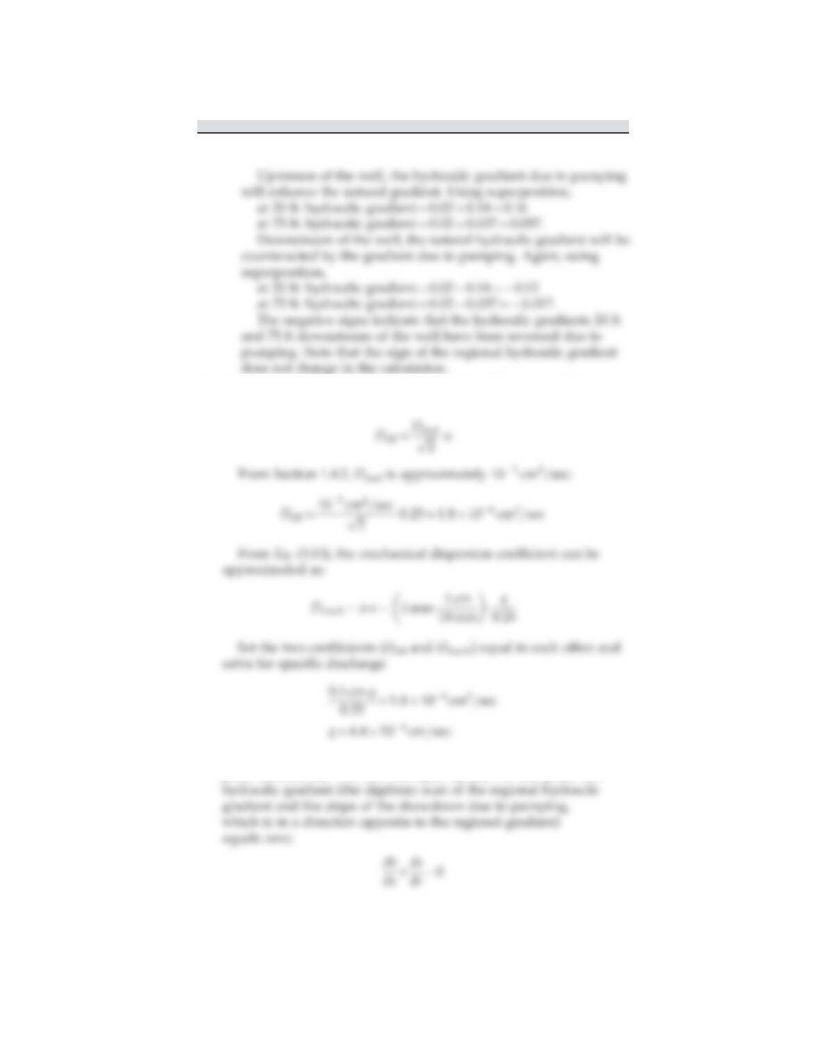
3. From Section 3.2.5, the effective molecular diffusion coefficient can
be approximated as:
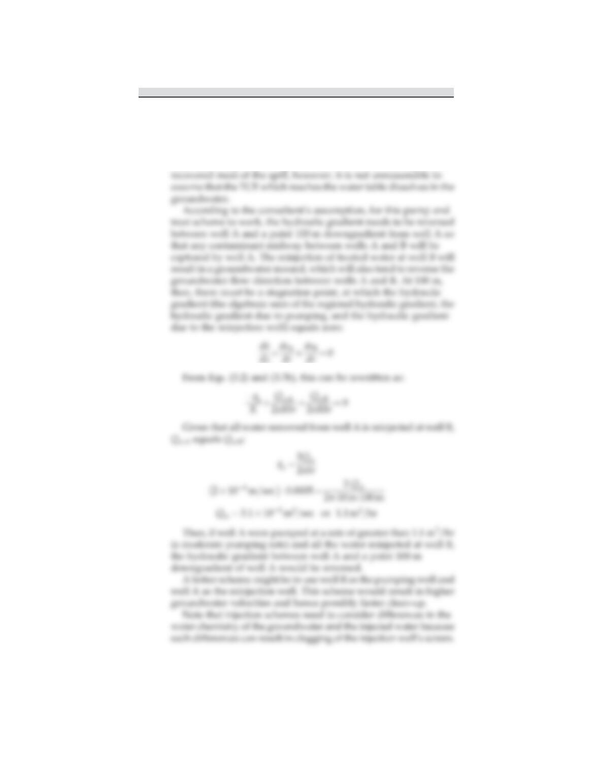
4. To avoid capturing any septic effluent, there must be a stagnation
point between the well and the septic system. At that point the
e68 SOLUTIONS MANUAL ONLINE
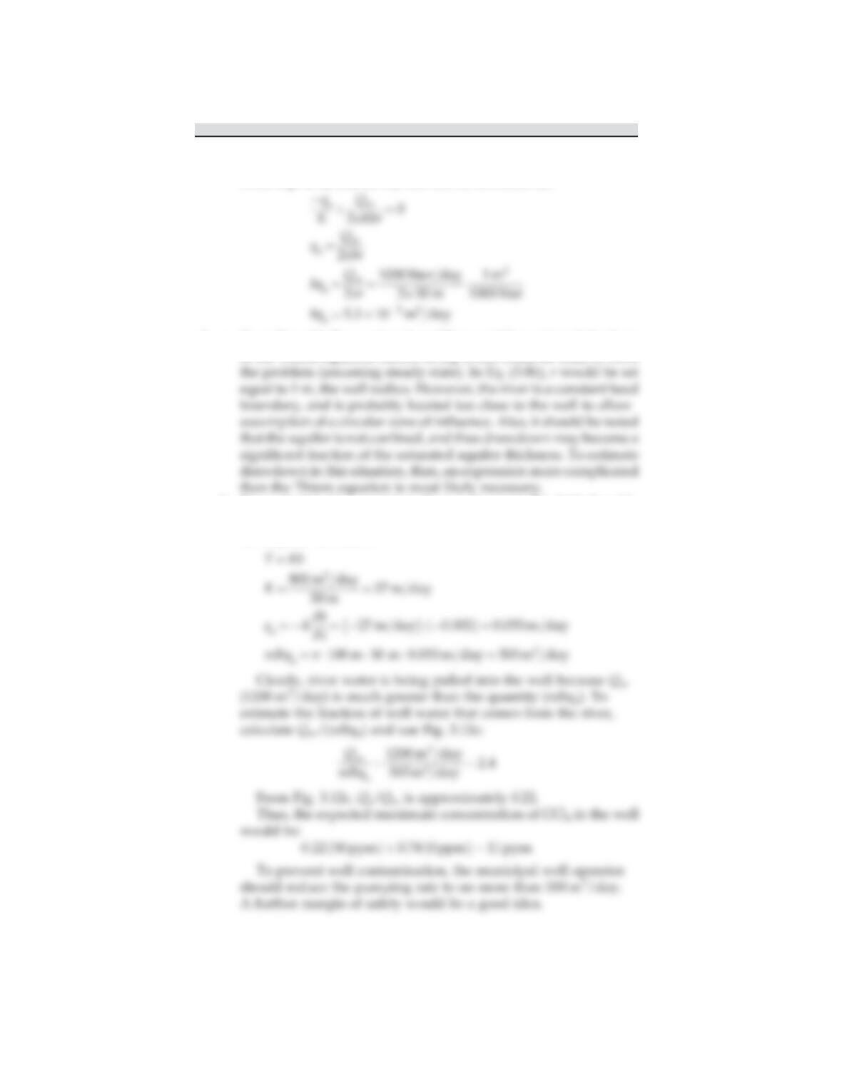
From Eqs. (3.2) and (3.7b), this can be rewritten as:
5. a. If a radius of influence less than 100 m could be assigned, the form
of the Thiem equation shown in Eq. (3.8b) could be used to solve
b. First calculate the quantity (pdbq
a
) as shown in Fig. 3.12. Specific
discharge (q
a
) can be estimated using data on transmissivity
and aquifer thickness:
e69CHAPTER 3 SOLUTIONS
6. a. To estimate the aquifer hydraulic conductivity, the form of the
Thiem equation shown in Eq. (3.8a) can be used. It is important to
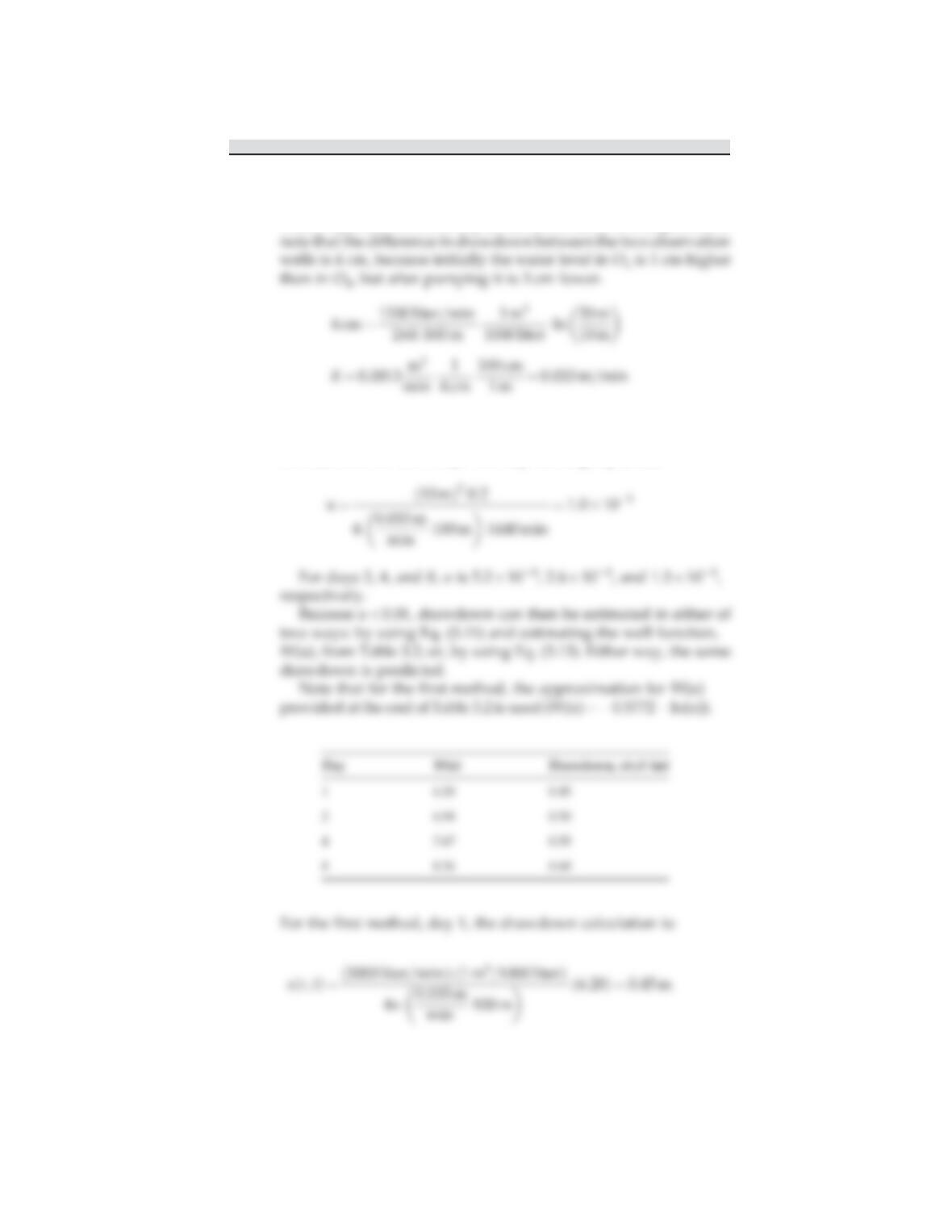
b. To tabulate drawdown versus time at observation well O
1
, the
Theis equation can be used. First, the well function variable umust
be estimated for the 5 days. For day 1, using Eq. (3.12):
e70 SOLUTIONS MANUAL ONLINE
7. The flow net provided shows no-flow boundaries along the bottom
and right-hand borders. Flow is shown as roughly parallel to these
boundaries. The upper border is a constant head at street level of
e71CHAPTER 3 SOLUTIONS
8. The breakthrough curve in a one-dimensional column is the plot of
chemical concentration at a fixed location as a function of time. The
rate of tracer movement will be the seepage velocity (Eq. 3.5),
assuming the tracer is ideal:
e72 SOLUTIONS MANUAL ONLINE
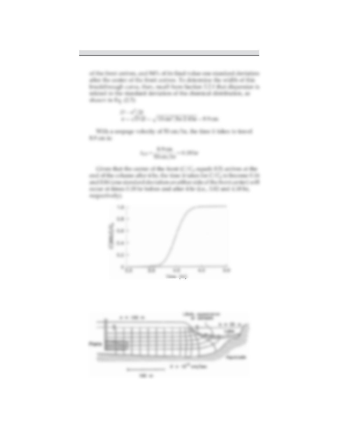
9. The flow net shown below indicates where the solvents are likely to
appear in the lake bed. Note that the area delineated assumes that no
dispersion of the plume occurs in the vertical direction.
e73CHAPTER 3 SOLUTIONS
To roughly approximate how long it will take for solvents traveling
with the water to reach the lake bed, use Eqs. (3.2) and (3.5). From the
flow net, the distance between the well and the lake bed along the
10. Some sorption of benzene to the organic carbon of the wetland soil
will occur, thus retarding the movement of benzene relative to the
e74 SOLUTIONS MANUAL ONLINE
11. First calculate the pseudo-first-order rate constant k0
12. The Theis equation can be used to determine the drawdown 5 m from
the well when the pumping is stopped. First estimate the well
function variable ufrom Eq. (3.12):
e75CHAPTER 3 SOLUTIONS
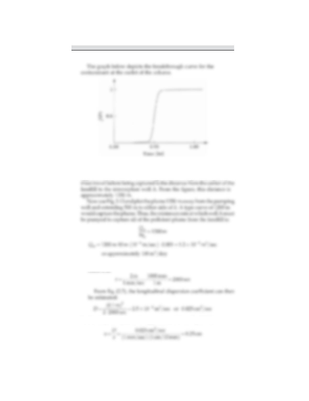
13. Given that the contaminant is injected into the column at a constant
concentration, Eq. (3.18) is the appropriate equation to use to describe
the contaminant concentration as a function of time at the outflow.
Given that the contaminant is nonsorbing, and assuming its decay is
negligible, the exponential decay term, e
kt
, can be set equal to one in
Eq. (3.18).
To estimate the seepage velocity, specific discharge must first be
estimated:
Using Eq. (3.5):
e76 SOLUTIONS MANUAL ONLINE
14. Assume the width of the pollutant plume can be approximated by the
width of the landfill. From the figure, the width of the landfill is
approximately 1000 m. The average distance the pollutant plume
15. a. First calculate the travel time for the center of tracer mass to
reach 2 m:
b. The dispersivity acan be approximated from Eq. (3.15):
e77CHAPTER 3 SOLUTIONS
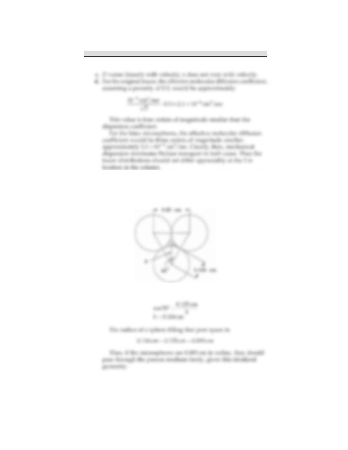
e. Assume the dispersivity of the aquifer estimated above in part (b)
is equal to the median grain diameter of the aquifer solids. Also
assume the grains are spherical and packed as tightly together as
possible, as shown below:
From the figure, the distance hcan be calculated as:
e78 SOLUTIONS MANUAL ONLINE
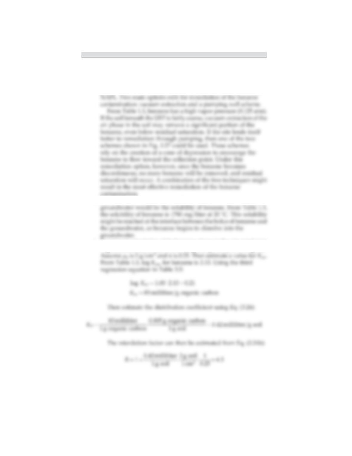
16. a. First estimate a value for the organic carbon-water partition
coefficient. From Table 1.3, log K
ow
¼1.97. Using the first
regression equation in Table 3.5:
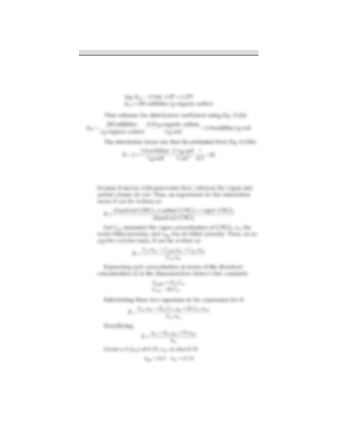
b. To calculate a retardation factor in unsaturated soil, consider the
generic definition of a retardation factor, presented in Eq. (3.22). In
the unsaturated soil, the dissolved CHCl
3
is considered mobile
e79CHAPTER 3 SOLUTIONS
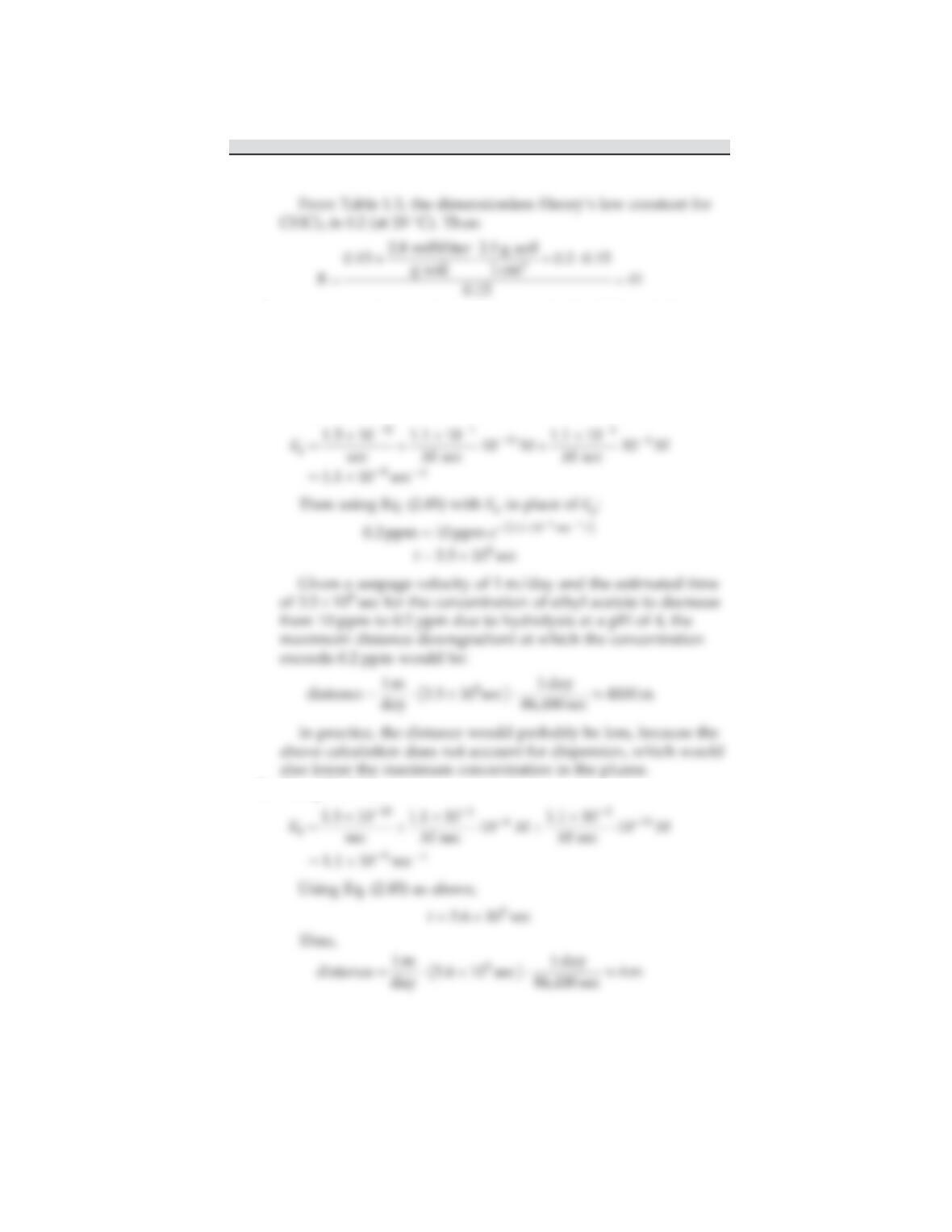
17. The maximum distance downgradient of the landfill at which a
concentration of ethyl acetate in excess of 0.2 ppm could be expected
depends primarily on the rate at which ethyl acetate degrades.
Assuming that ethyl acetate degrades only through hydrolysis, use
the hydrolysis rates presented in Table 2.13 and Eq. (2.89):
a. At a pH of 4,
b. At a pH of 10,
e80 SOLUTIONS MANUAL ONLINE
18. a. Benzene will float on the water table below the underground
storage tank (UST) because benzene is a NAPL. There is a high
probability of recovering a significant fraction of the benzene as
contamination.
b. The maximum concentration of benzene that could occur in the
c. To estimate retardation of the benzene plume in the saturated zone
requires estimates of the bulk density and porosity of the aquifer.
e81CHAPTER 3 SOLUTIONS
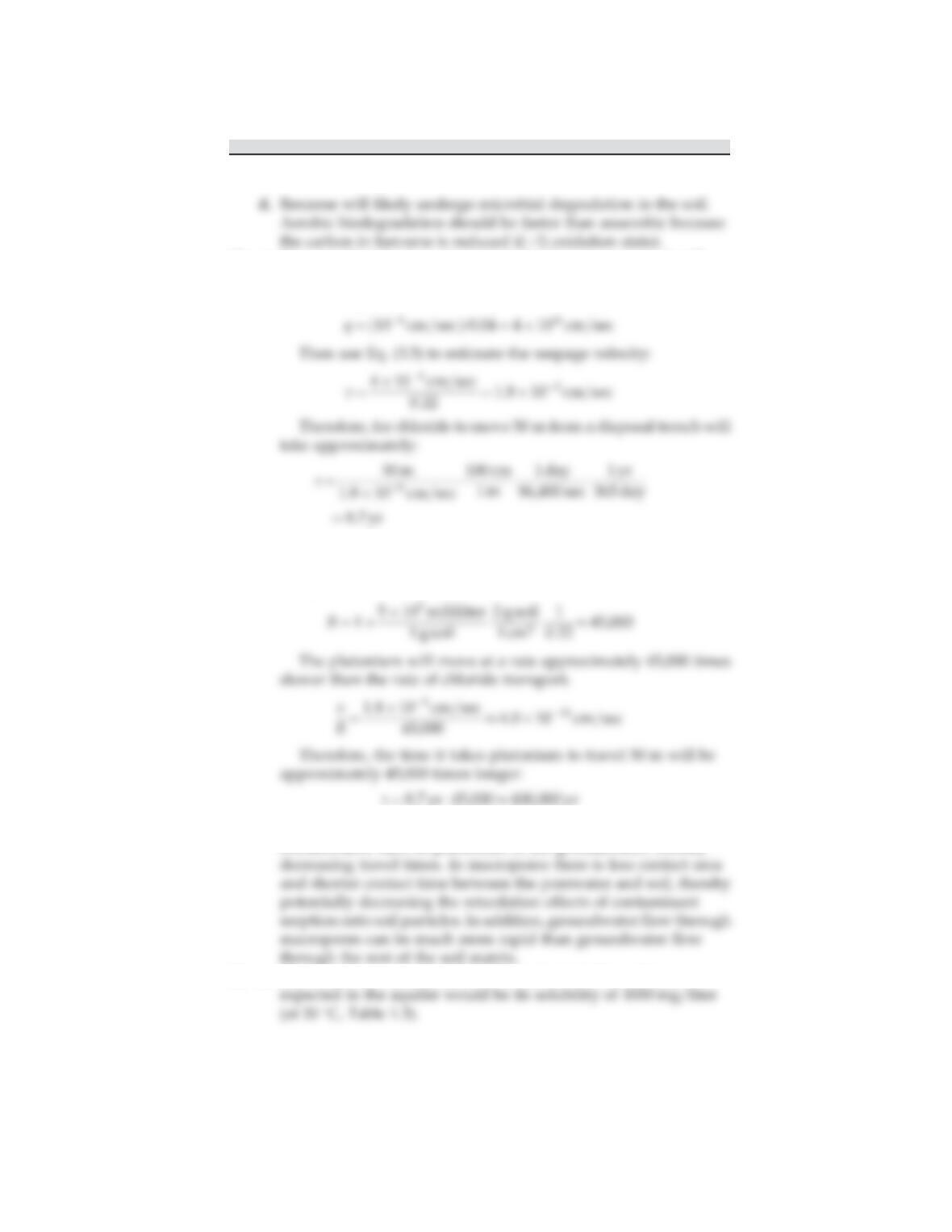
19. a. Because chloride approximates an ideal tracer, assume it will
move through the soil without retardation at the seepage velocity.
First use Eq. (3.2) to estimate specific discharge:
b. To estimate how long it will take for plutonium to move 50 m, a
retardation factor must be estimated. Assuming a soil bulk density
of 2 g/cm
3
and using Eq. (3.24b):
c. The presence of macropores can greatly enhance the transport of
contaminants such as plutonium in the groundwater, thereby
20. a. The maximum concentration of dissolved trichloroethene
e82 SOLUTIONS MANUAL ONLINE
b. TCE is a DNAPL. If sufficient quantities entered the groundwater,
a separate phase might be maintained and the TCE could sink to
the bottom of the aquifer and potentially enter fractures in the
bedrock, as depicted in Fig. 3.25. Given that the clean-up crews
e83CHAPTER 3 SOLUTIONS
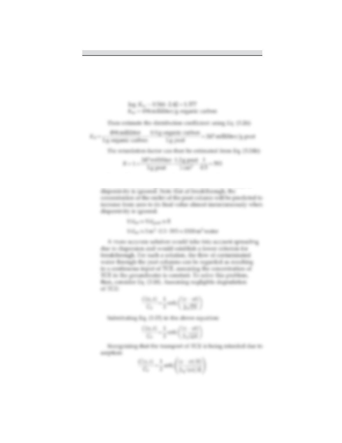
c. The peat columns are treating the groundwater by sorbing the
TCE. First calculate a retardation factor for TCE. From Table 1.3,
log K
ow
for TCE is 2.42. Use the first regression equation in
Table 3.5 to estimate K
oc
:
To roughly estimate the volume of water each peat column can
treat until breakthrough, a simple calculation can be made if
e84 SOLUTIONS MANUAL ONLINE
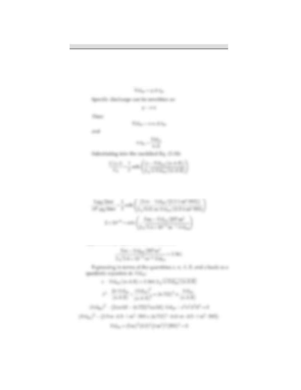
Water flows through the column at a specific discharge q
(Eq. 3.2). Thus, the volume of water treated (Vol
trt
) equals the
specific discharge multiplied by the cross-sectional area and the
time until breakthrough (t
bt
):
To solve this equation requires a judgment as to what TCE
concentration constitutes breakthrough. Assume that C(5 m, t
bt
)¼
1mg/liter is considered breakthrough:
Using Eq. (3.19) and a sufficient number of terms, erfc (3.361)
approximately equals 210
6
. Therefore:
e85CHAPTER 3 SOLUTIONS
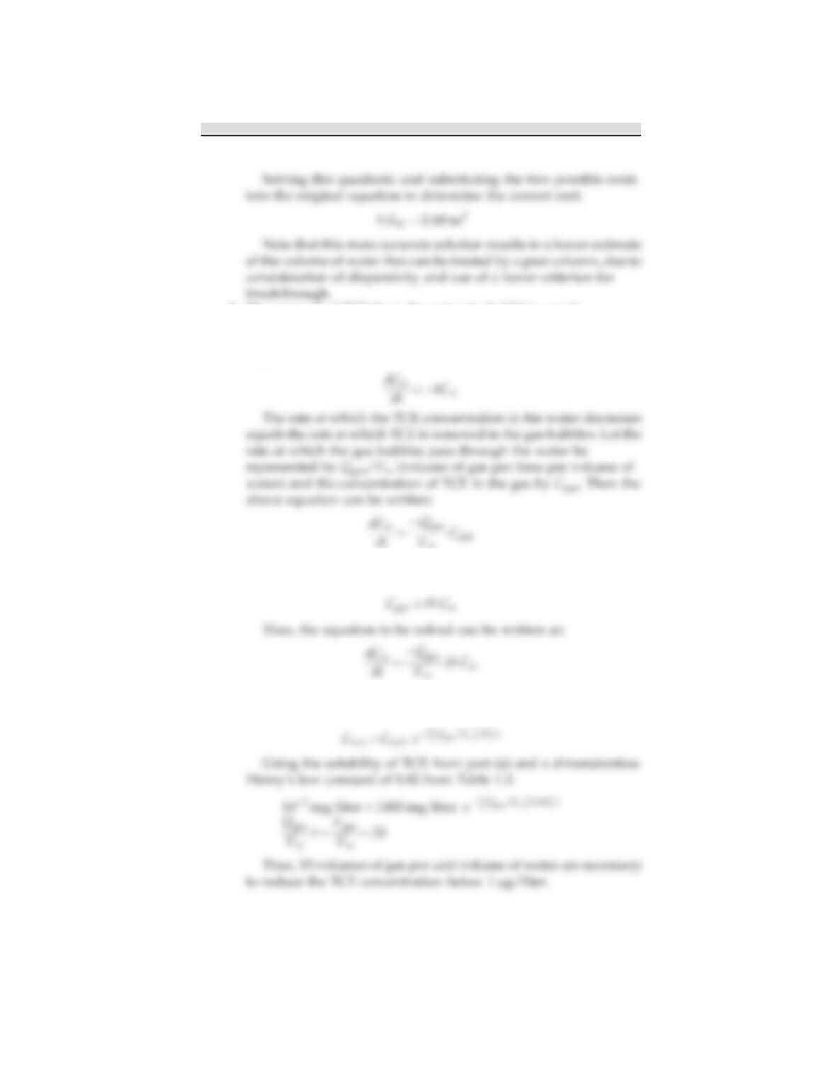
d. The removal of TCE from the water by bubbling can be
approximated as a first-order removal process. Referring to
Eq. (1.19) and letting C
w
represent the concentration of TCE in the
water:
The concentration of TCE in the gas will depend on the Henry’s
law constant (H):
The solution to this first-order decay equation (refer to Eq. 1.20)
is:
e86 SOLUTIONS MANUAL ONLINE