75
Groundwater Dating
1. Give examples of radiometric dating methods involving (i) loss of parent, (ii) ingrowth of daughter,
and (iii) both loss of parent and gain of daughter.
(i) Tritium decay to 3He, using residual tritium as an indication of age. This is not
quantitative due to the variable history of tritium in precipitation
2. The following noble gas concentrations were measured for low-salinity coastal aquifer groundwaters
which were dated with radiocarbon to 22,000 years before present. Correct for excess air with Ne and
calculate an estimate for the paleo-groundwater recharge temperature.
a) Ne = 3.08 ·10 7 ccSTP/ccH2O
b) Kr = 1.13 ·10 7 ccSTP/ccH2O
c) Xe = 1.63 ·10 8 ccSTP/ccH2O
These three noble gases have different solubilities and are all atmospherically derived. Their
dissolved concentrations will therefore reflect the recharge temperature, but first must be corrected
for the common input from excess air (see Noble Gas Recharge Temperatures on page 283).
8
76
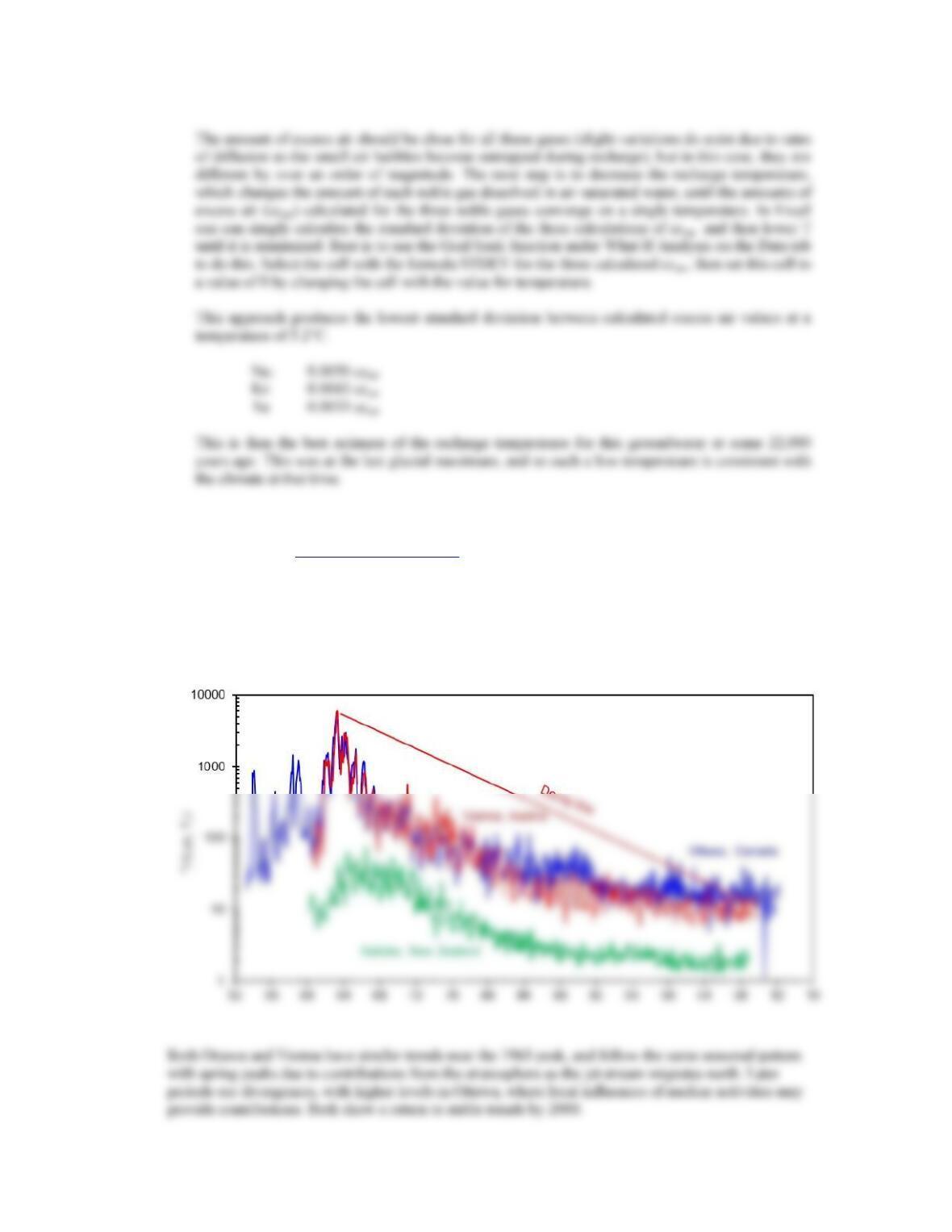
3. Visit the GNIP site (http://www.iaea.org/water) and download tritium data from Ottawa (Canada),
Vienna (Austria), and Kaitoke (New Zealand). Plot these data on a semilogarithmic chart. Account for
the similarities and/or differences in the magnitude of the 1963 thermonuclear peaks in these records.
Why do all records have strong seasonal variability? Plot decay curves on the chart. What are the two
principal factors contributing to the attenuation of the high levels of tritium from 1963 to today? What
are the constraints on using this 1963 peak in groundwater as a time horizon for dating?
77
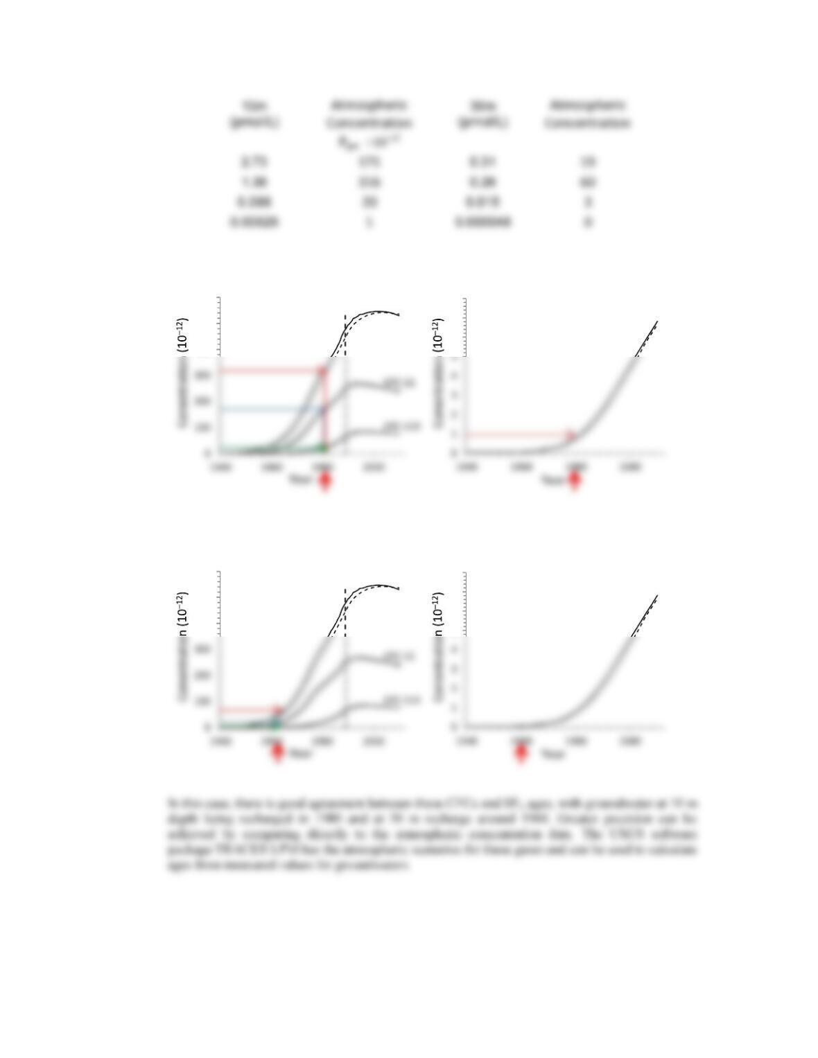
4. The following CFC and SF6 measurements were made for 15°C groundwater sampled in a
semiconfined sand aquifer in southern Ontario. Calculate the atmospheric concentrations of these
compounds and compare with the atmospheric scenarios in Fig. 8-3 to determine a mean subsurface
residence time for these samples. Concentrations are parts per trillion (10 12 or xmol/L) in
groundwater.
CFC-11
CFC-12
CFC-113
SF6
10m (pmol/L) 2.73
1.36
0.098
0.00026
30m (pmol/L) 0.31
0.26
0.015
0.000048
K
H
15°C (pmol/L/atm) 0.016
0.0043
0.0049
0.00032
These constants are used to calculate the atmospheric partial pressure of the gas in the atmosphere,
according to:
KH gas =
78
10 m
30 m
400
500
600
CFCs
Montreal
Protocol CFC-12
6
7
8
SF6
400
500
600
CFCs
Montreal
Protocol CFC-12
5
6
7
8
SF6
79
5. A sample of groundwater sampled June 21, 2009 was not analyzed for tritium until November 13,
2013 due to technical problems. The measured value was 6.8 TU. What was its tritium concentration
on the sampling date?
The tritium concentration on the sampling date is the relevant value for any calculation of
groundwater age. Unlike radiocarbon, the short half-life of tritium causes a decrease in activity of
about 5.6% per year, which is derived from the decay equation:
6. Groundwater from the base of an alluvial aquifer overlying crystalline bedrock had a helium
concentration (corrected for excess air) of 1.47×10 7 ccSTP/ccH2O and a recharge temperature of 15°C.
sample for dating by the T–3He method?
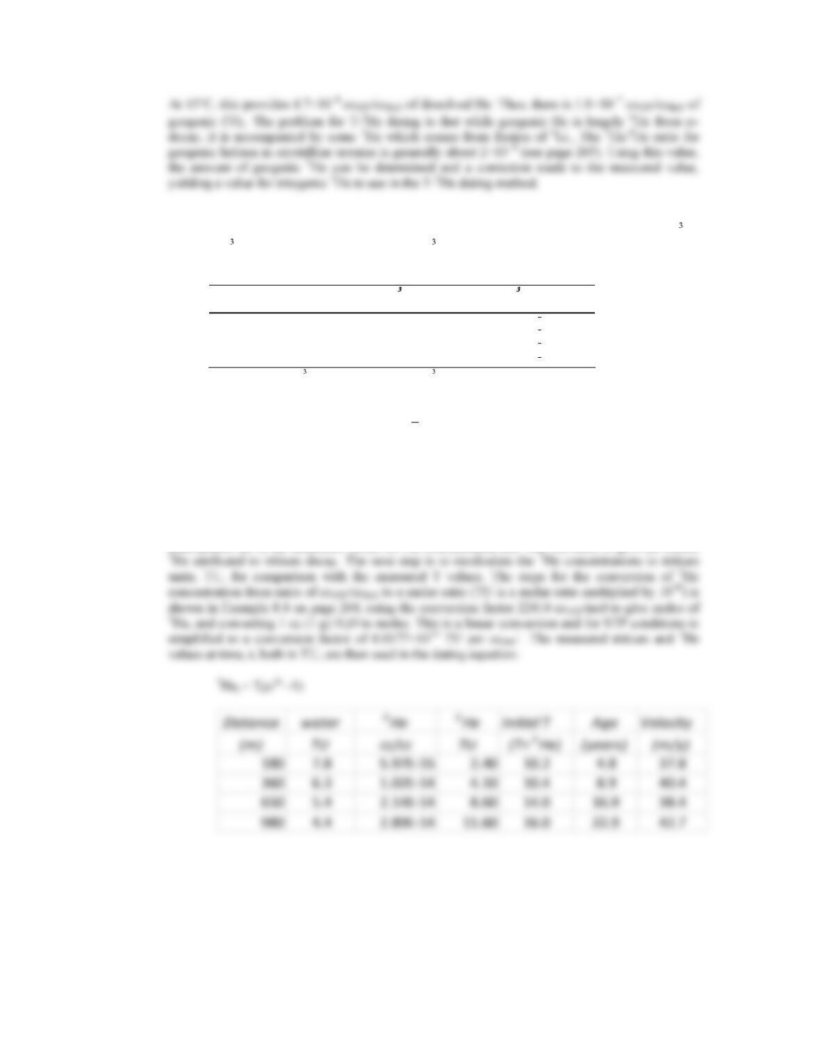
The measured He, here corrected for excess air, is 1.47×10 7 ccSTP/ccH2O. The contribution derived
from dissolution of atmospheric helium is determined from the equation in Figure 8.12:
80
7. A series of shallow groundwaters (10°C) were sampled from a confined sandy aquifer from
piezometers installed at increasing distances from the unconfined recharge area. Analysis of T and He
concentrations ( He values corrected for atmospheric He) gave the following results:
Sample Distance from
recharge (m) H (TU) He
(ccSTP/ccH2O)
CJ1 180 7.8 5.97×10
15
CJ2 360 6.3 1.02×10
14
CJ3 650 5.4 2.14×10
14
CJ4 980 4.4 2.89×10
14
Conversion: 1 ccSTP He/ccH2O = 4.0177×10¹⁴ TU ( He equivalent)
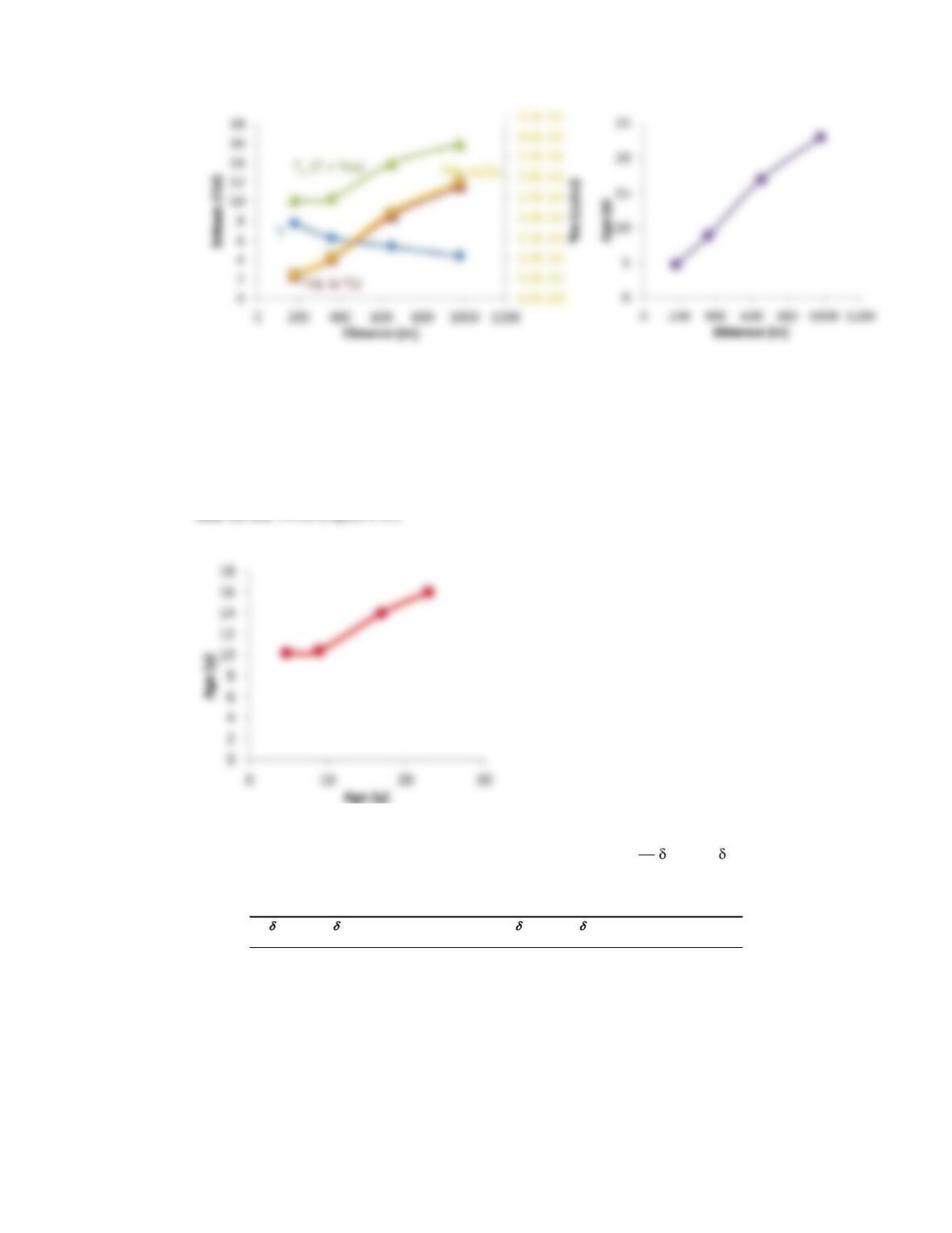
Plot the distribution of T and 3He with distance from the recharge area, with 3He both in units of
ccSTP/ccH2O and in equivalent TU. Calculate the T 3He age for each sample and from this calculate the
average groundwater velocity (note that the calculated ages will be a mean of a range due to
hydrodynamic dispersion). What was the initial tritium concentration in each sample at the time of
recharge? Plot initial tritium with age for each sample and account for the change through time. (Refer
to the charts in Figures 8.5 and 8.10 and suggest possible regions where this aquifer may be located.)
In this problem, the helium data has already been corrected for excess air and dissolved
atmospheric He in the measured values for He concentration and 3He/4He ratio, to give the excess
81
Plotting initial tritium with age is done by simply adding the measured remaining tritium in a
sample with the tritogenic or daughter 3H. This gives the initial tritium concentration before decay
starts (t =0 and 3He = 0). In this plot, we see that the youngest samples have the lowest (and
stable) initial tritium concentrations indicating a steady input function. This is close to that
measured today in high latitude regions such as Europe (see the trend for Vienna in Figure 8.10).
The older samples have higher initial tritium which is likely related to the residual anthropogenic
tritium from atmospheric testing of nuclear bombs, which was present in precipitation globally
until the late 1990s (Figure 8.10)
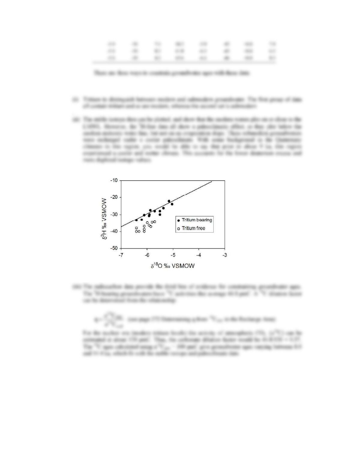
8. Groundwaters were sampled from a Cretaceous limestone aquifer (LMWL D = 7.8 18O + 10) and
have produced the following data. What are the age constraints given by the stable isotope data and
from the tritium data and from the radiocarbon data?
18O
2H
3
H
TU
14
C
pMC
18O 2H
3
H
TU
14
C
pMC
–
5.9
–
36
9.4
40.1
–
5.7
–
42
<0
.8
14.1
–
6.1
–
38
6.5
45.3
–
6.1
–
46
<0.8
12.2
–
6.2
–
40
2.5
39.6
–
5.9
–
43
<0.8
9.5
–
5.7
–
34
6.7
43.9
–
6.0
–
41
<0.8
8.9
–
5.4
–
32
8.3
51.1
–
6.4
–
44
<0.8
9.6
–
5.9
–
37
9.6
46.4
–
6.1
–
43
<0.8
7.1
–
5.5
–
34
5.8
44.7
–
6.3
–
46
<0.8
12.8
–
5.5
–
35
6.9
45.8
-5.
8
–
41
<0.8
10.5
–
6.2
–
38
8.1
52.2
–
6.1
–
45
<0.8
10.2
82
9. The following analysis was carried out on a groundwater from a carbonate aquifer. Assume that the Ca
+ Mg accurately reflect the total amount of calcite dissolved and that Ca + Mg was modified by
evaporite dissolution and ion exchange (i.e. Na and Cl should be balanced, differences reflect ion
exchange) (concentrations in mg/L):
83
pH T HCO
3
SO
4
2 Cl Na+ Ca2+ Mg2+
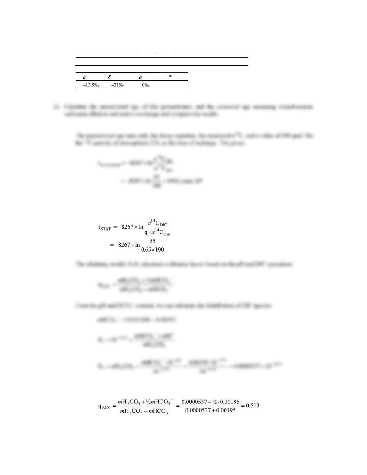
7.91 25°C 119 1.2 8.9 17.0 25 2.8
13CDIC 13Csoil-CO
2
13Ccarb CDIC
55 pMC
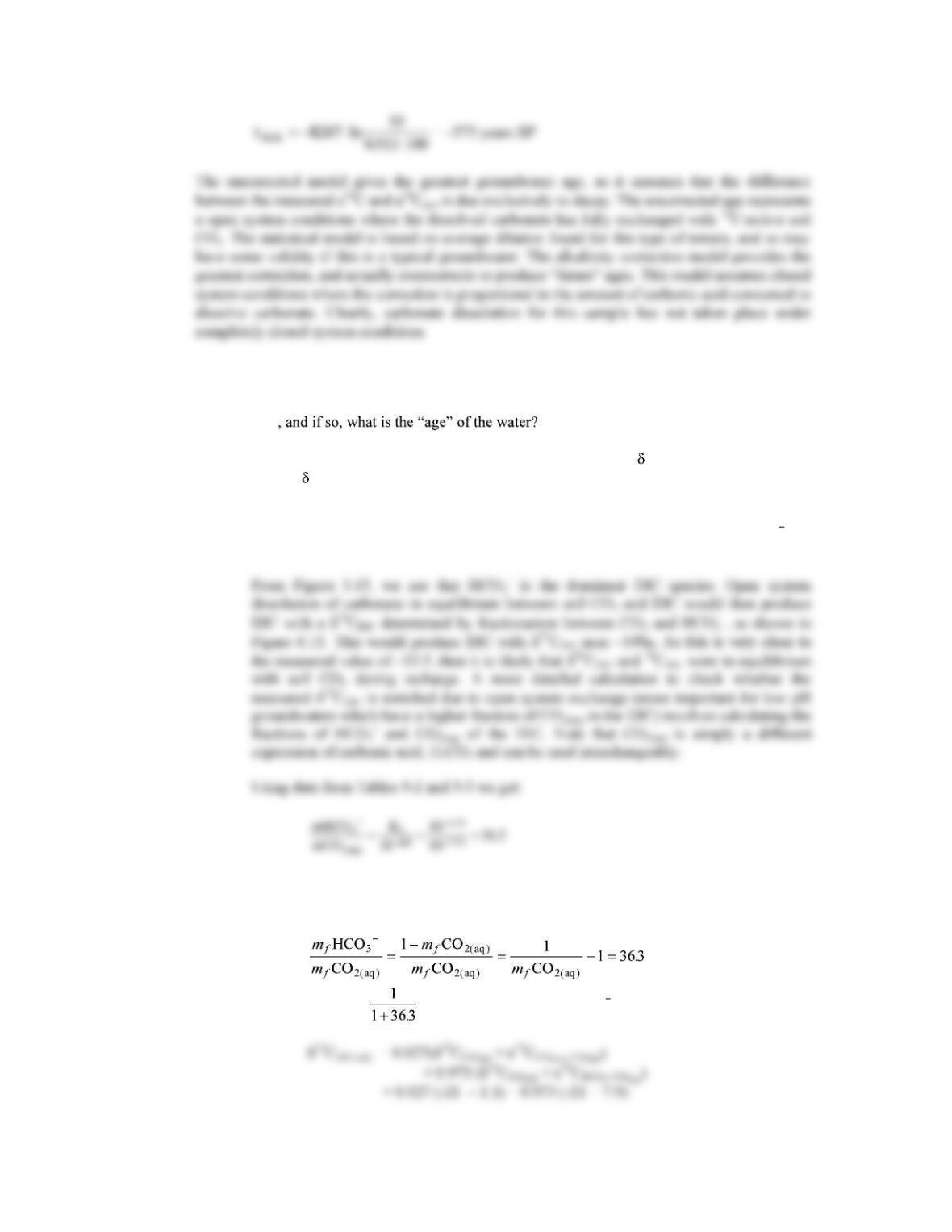
The statistical correction model applies a dilution factor of 0.5 to 0.75 for karst or carbonate
systems. Using a median value of say 0.65, we get:
= 1381 years BP
The dilution factor is then:
84
(ii) Could these results be explained as an open system for CO2 uptake and calcite dissolution (in
which case 14CDIC is undiluted as it has exchanged with soil CO2 during carbonate dissolution and,
and so q is 1)
The open system condition can be tested by calculating the 13CDIC value for the given
pH and 13C of the soil. Recall that during open system carbonate dissolution, exchange
with the soil CO2 dominates and so the isotopic composition of the carbonate does not
influence the DIC. First, use pH to determine the distribution of carbonate species that
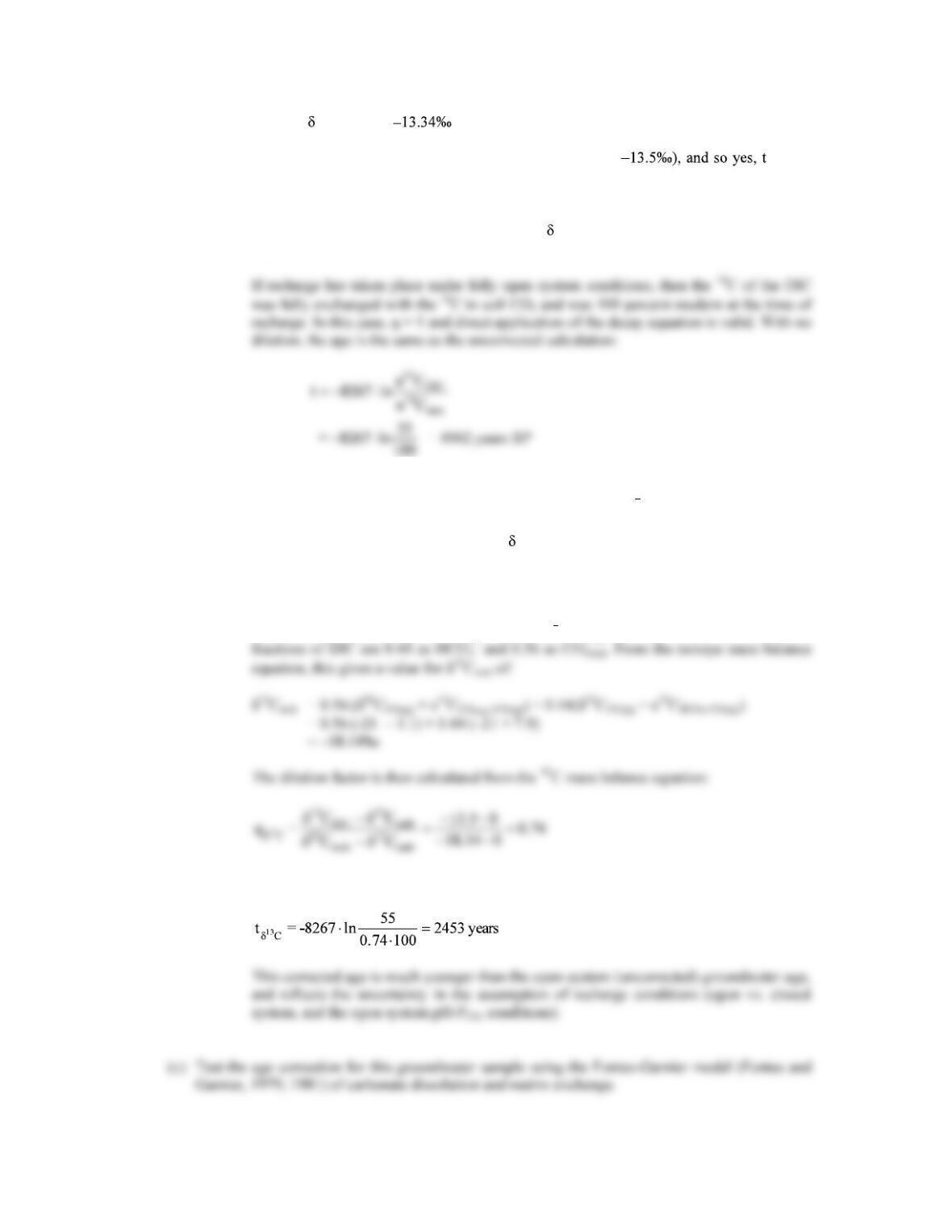
exchange with the CO2. The pH is less than 8.4 and so only CO2(aq) and HCO3 are
important.
and using mole fractions (mf):
mfCO2(aq) + mfHCO3 = 1
Thus, mfCO2(aq) = = 0.027 and mHCO3 = 0.973
85
13CDIC-calc =
This value is essentially the same as the measured value ( his can
be explained by open system conditions. However, one must be careful because this
assumes that the measured pH and the carbonate system have not evolved during the
residence time of this groundwater in the saturated zone of the aquifer. If the pH was
lower in the recharge area, then this calculated 13CDIC would be lower than the measured
value.
(iii) Assume that a pH of 6.25 and DIC of 0.96 mmoles (at PCO2 = 10 1.8) were measured for the
infiltrating groundwaters in the recharge area, prior to closed system dissolution of calcite.
Calculate the age of these groundwaters using the 13C mixing model.
In this case carbonate dissolution begins under open system conditions in the soil zone
but reaches calcite saturation under closed system conditions below the water table. The
distribution of DIC species is calculated in the same way as in (ii) only using pH 6.25
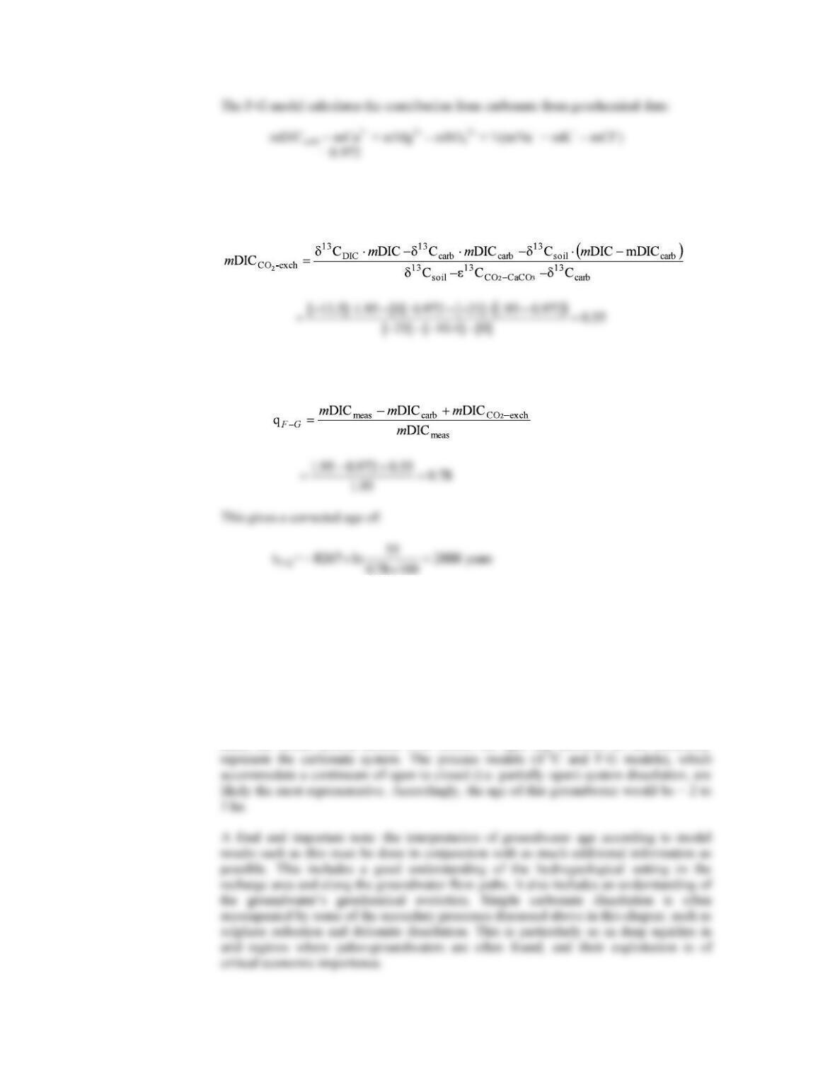
instead of the measured pH. This gives a HCO3/CO2(aq) ratio of 0.79, and so the relative
Using this dilution factor, we get a corrected age of:
86
This model then calculates how much of this carbonate has exchanged with the soil CO2
under open system conditions, using a 13C mass balance:
The dilution factor is then calculated from these various proportions of DIC:
The Fontes-Garnier model is often the most representative as it does not require any
estimates of the pH and PCO2 conditions in the open-system recharge environment. It uses
only the measured pH and DIC values and the model of carbonate dissolution to calculate
a dilution factor. Thus, it accounts for both open system and closed system carbonate
dissolution.
The uncorrected age, assuming fully open system dissolution of carbonate is unlikely to
represent this groundwater. Such conditions are exceptional and additional reaction
through matrix exchange or dolomite dissolution are not taken into account. On the other
hand, the closed system models over correct the ages and therefore do not accurately
87
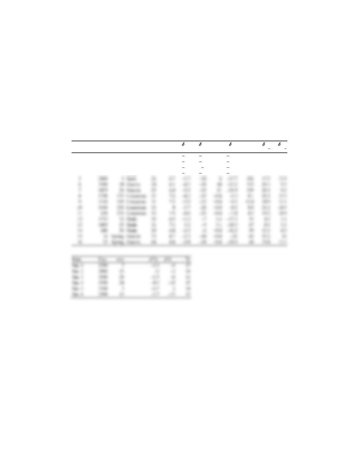
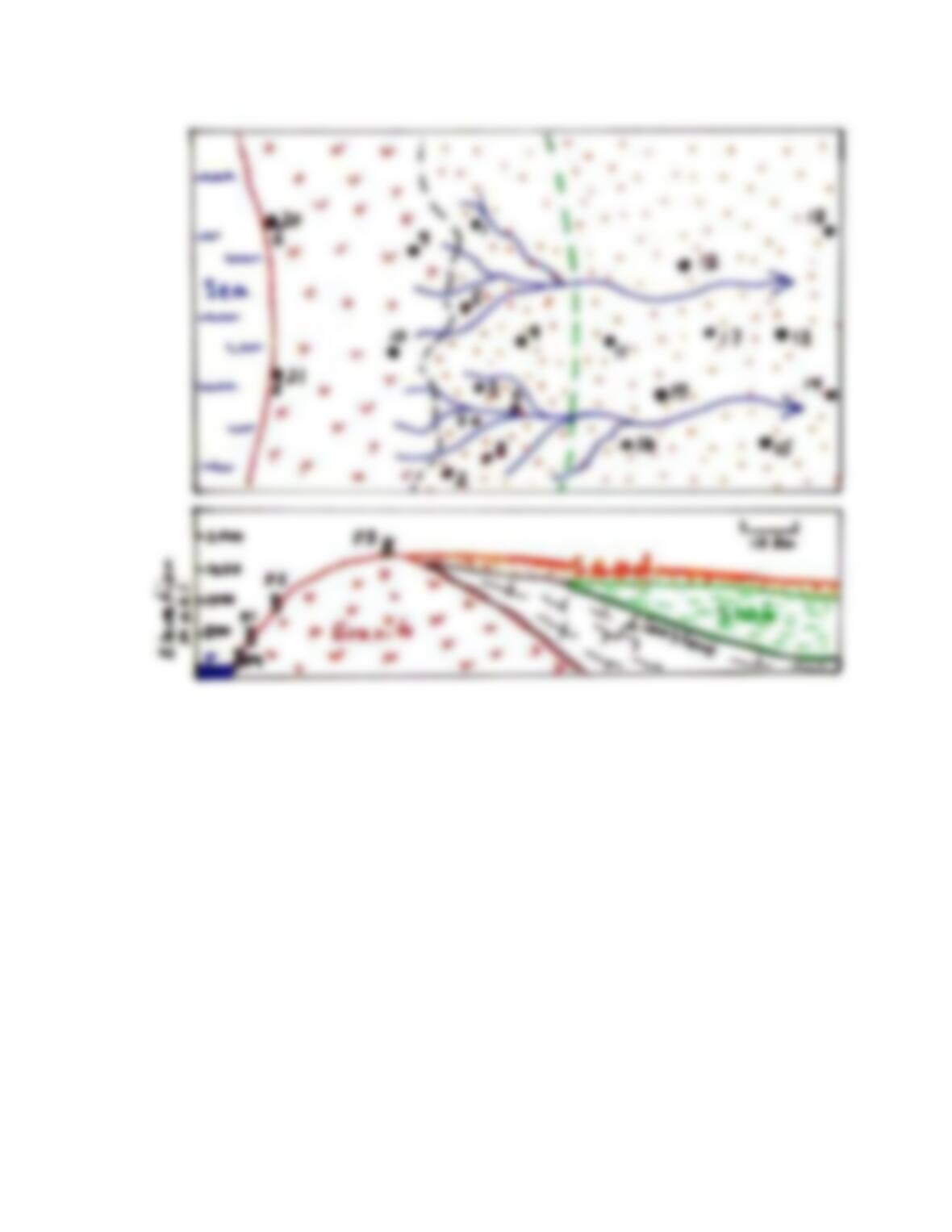
10. The following data have been produced from analyzing groundwaters and precipitation sampled from
sites given on the adjoining map. Field data is given on this table with the isotope data. Your task is to
evaluate these data and provide a brief but informative report with respect to the recharge origin and
subsurface mean residence times of these groundwaters. In your evaluation, include relevant graphs as
interpretive tools and to support your observations. In your report, note any assumptions you use in
your interpretations.
There are interesting and interpretable trends in the data. Treat this as a real problem and discuss
your interpretations with your fellow students and instructor.
Sample
Elevation
Depth
Rock type
Temp
pH
18
O
2
H
3
H
13
C
a
14
C
34
S
18
O
m a.s.l.
°C
pmC
SO4
2
SO4
2
1
2510
8
Sand 27
6.6
2.5
20
7
18.1
117
15
.1
17.2
2
2500
15
Limestone
26
7.3
2.0
15
15
13.3
83
17.5
14.8
3
2450
18
Limestone
27
7.5
1.9
5
9
12.5
87
19.8
13.7
4
2710
7
Sand 25
6.9
3.1
22
12
17.9
123
17
15.9
2800
9
6.7
1.7
18
6
17.7
104
17.5
13.9
3500
28
6.1
4.3
20
48
23.2
125
20.3
9.5
3475
21
6.4
3.5
15
21
21.9
119
20.1
9.2
1790
175
7.6
4.2
25
<0.8
5.3
8.1
20.5
15.5
1320
195
7.5
3.9
23
<0.8
9.1
12.8
18.9
13.1
1010
230
8
3.7
20
<0.8
.2
8.8
21.1
14.5
630
275
7.9
4.0
23
<0.8
7.8
4.5
19.2
14.9
1715
32
6.9
1.2
7
1.4
17.1
55
4.2
1.1
1405
25
7.1
0.2
5
3.1
18.3
67
8.1
3.2
680
19
6.8
0.5
6
<0.8
16.5
59
12.1
4.3
16
Spring
8.7
2.3
18
<0.8
23
62
21.2
14
25
Spring
8.4
2.8
18
<0.8
20.9
68
19.8
13.2
Elev.
H
2500
7
1.3
5
17
2800
25
2
2
10
3000
29
2.5
6
11
3500
24
4.3
19
15
3100
3
0.7
2
14
2900
22
3.7
15
15
88